Main Content
Syntax
Description
Examples
collapse all
Find Error Function
Find the error function of a value.
Find the error function of the elements of a vector.
V = [-0.5 0 1 0.72];
erf(V)
ans = 1×4

   -0.5205         0    0.8427    0.6914
Find the error function of the elements of a matrix.
M = [0.29 -0.11; 3.1 -2.9];
erf(M)
ans = 2×2

    0.3183   -0.1236
    1.0000   -1.0000
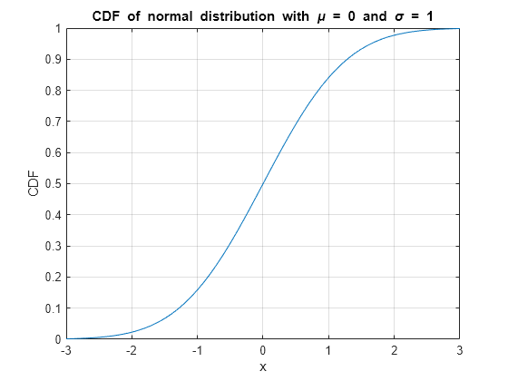
Find Cumulative Distribution Function of Normal Distribution
The cumulative distribution function (CDF) of the normal, or Gaussian, distribution with standard deviation σ and mean μ is
ϕ(x)=12(1+erf(x-μσ2)).
Note that for increased computational accuracy, you can rewrite the formula in terms of erfc . For details, see Tips.
Plot the CDF of the normal distribution with μ=0 and σ=1.
x = -3:0.1:3;
y = (1/2)*(1+erf(x/sqrt(2)));
plot(x,y)
grid on
title('CDF of normal distribution with mu = 0 and sigma = 1')
xlabel('x')
ylabel('CDF')
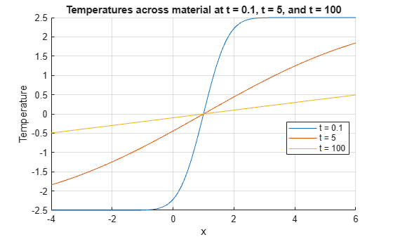
Calculate Solution of Heat Equation with Initial Condition
Where u(x,t) represents the temperature at position x and time t, the heat equation is
∂u∂t=c∂2u∂x2,
where c is a constant.
For a material with heat coefficient k, and for the initial condition u(x,0)=a for x>b and u(x,0)=0 elsewhere, the solution to the heat equation is
u(x,t)=a2(erf(x-b4kt)).
For k = 2, a = 5, and b = 1, plot the solution of the heat equation at times t = 0.1, 5, and 100.
x = -4:0.01:6;
t = [0.1 5 100];
a = 5;
k = 2;
b = 1;
figure(1)
hold on
for i = 1:3
    u(i,:) = (a/2)*(erf((x-b)/sqrt(4*k*t(i))));
    plot(x,u(i,:))
end
grid on
xlabel('x')
ylabel('Temperature')
legend('t = 0.1','t = 5','t = 100','Location','best')
title('Temperatures across material at t = 0.1, t = 5, and t = 100')
Input Arguments
collapse all
x — Input
real number | vector of real numbers | matrix of real numbers | multidimensional array of real numbers
Input, specified as a real number, or a vector, matrix, or multidimensional
array of real numbers. x cannot be sparse.
Data Types: single | double
More About
collapse all
Error Function
The error function erf of x is
Tips
-
You can also find the standard normal probability
distribution using the functionnormcdf(Statistics and Machine Learning Toolbox). The relationship between the error
functionerfandnormcdfis -
For expressions of the form
1 - erf(x),
use the complementary error functionerfcinstead.
This substitution maintains accuracy. Whenerf(x)is
close to1, then1 - erf(x)is
a small number and might be rounded down to0.
Instead, replace1 - erf(x)witherfc(x).
Extended Capabilities
Tall Arrays
Calculate with arrays that have more rows than fit in memory.
This function fully supports tall arrays. For
more information, see Tall Arrays.
C/C++ Code Generation
Generate C and C++ code using MATLAB® Coder™.
Usage notes and limitations:
-
Strict single-precision calculations are not supported. In the
generated code, single-precision inputs produce single-precision
outputs. However, variables inside the function might be
double-precision.
Thread-Based Environment
Run code in the background using MATLAB® backgroundPool or accelerate code with Parallel Computing Toolbox™ ThreadPool.
This function fully supports thread-based environments. For
more information, see Run MATLAB Functions in Thread-Based Environment.
GPU Arrays
Accelerate code by running on a graphics processing unit (GPU) using Parallel Computing Toolbox™.
This function fully supports GPU arrays. For more information, see Run MATLAB Functions on a GPU (Parallel Computing Toolbox).
Distributed Arrays
Partition large arrays across the combined memory of your cluster using Parallel Computing Toolbox™.
This function fully supports distributed arrays. For more
information, see Run MATLAB Functions with Distributed Arrays (Parallel Computing Toolbox).
Version History
Introduced before R2006a
- Trial Software
- Trial Software
- Product Updates
- Product Updates
Complementary error function
Syntax
Description
Examples
Complementary Error Function for Floating-Point and Symbolic Numbers
Depending on its arguments, erfc can
return floating-point or exact symbolic results.
Compute the complementary error function for these numbers.
Because these numbers are not symbolic objects, you get the floating-point
results:
A = [erfc(1/2), erfc(1.41), erfc(sqrt(2))]
Compute the complementary error function for the same numbers
converted to symbolic objects. For most symbolic (exact) numbers, erfc returns
unresolved symbolic calls:
symA = [erfc(sym(1/2)), erfc(sym(1.41)), erfc(sqrt(sym(2)))]
symA =
[ erfc(1/2), erfc(141/100), erfc(2^(1/2))]
Use vpa to approximate symbolic results
with the required number of digits:
d = digits(10);
vpa(symA)
digits(d)
ans =
[ 0.4795001222, 0.04614756064, 0.0455002639]
Error Function for Variables and Expressions
For most symbolic variables and expressions, erfc returns
unresolved symbolic calls.
Compute the complementary error function for x and sin(x):
+ x*exp(x)
syms x
f = sin(x) + x*exp(x);
erfc(x)
erfc(f)
ans =
erfc(x)

ans =
erfc(sin(x) + x*exp(x))
Complementary Error Function for Vectors and Matrices
If the input argument is a vector or a matrix, erfc returns
the complementary error function for each element of that vector or
matrix.
Compute the complementary error function for elements of matrix M and
vector V:
M = sym([0 inf; 1/3 -inf]);
V = sym([1; -i*inf]);
erfc(M)
erfc(V)
ans =
[         1, 0]
[ erfc(1/3), 2]

ans =
    erfc(1)
 1 + Inf*1i
Compute the iterated integral of the complementary error function
for the elements of V and M,
and the integer -1:
ans =
[             2/pi^(1/2), 0]
[ (2*exp(-1/9))/pi^(1/2), 0]

ans =
 (2*exp(-1))/pi^(1/2)
                  Inf
Special Values of Complementary Error Function
erfc returns special values
for particular parameters.
Compute the complementary error function for x =
0, x =
∞, and x =
–∞. The complementary error function has special
values for these parameters:
[erfc(0), erfc(Inf), erfc(-Inf)]
Compute the complementary error function for complex infinities.
Use sym to convert complex infinities to symbolic
objects:
[erfc(sym(i*Inf)), erfc(sym(-i*Inf))]
ans =
[ 1 - Inf*1i, 1 + Inf*1i]
Handling Expressions That Contain Complementary Error Function
Many functions, such as diff and int,
can handle expressions containing erfc.
Compute the first and second derivatives of the complementary
error function:
syms x
diff(erfc(x), x)
diff(erfc(x), x, 2)
ans =
-(2*exp(-x^2))/pi^(1/2)

ans =
(4*x*exp(-x^2))/pi^(1/2)
Compute the integrals of these expressions:
syms x
int(erfc(-1, x), x)
ans =
x*erfc(x) - exp(-x^2)/pi^(1/2)
ans =
(x^3*erfc(x))/6 - exp(-x^2)/(6*pi^(1/2)) +...
(x*erfc(x))/4 - (x^2*exp(-x^2))/(6*pi^(1/2))
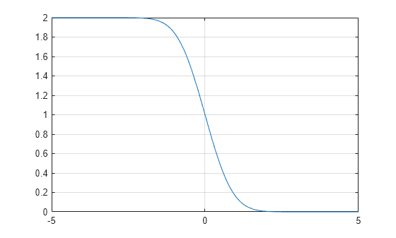
Plot Complementary Error Function
Plot the complementary error function on the interval from -5 to 5.
syms x
fplot(erfc(x),[-5 5])
grid on
Input Arguments
collapse all
X — Input
symbolic number | symbolic variable | symbolic expression | symbolic function | symbolic vector | symbolic matrix
Input, specified as a symbolic number, variable, expression,
or function, or as a vector or matrix of symbolic numbers, variables,
expressions, or functions.
K — Input representing an integer larger than -2
number | symbolic number | symbolic variable | symbolic expression | symbolic function | symbolic vector | symbolic matrix
Input representing an integer larger than -2,
specified as a number, symbolic number, variable, expression, or function.
This arguments can also be a vector or matrix of numbers, symbolic
numbers, variables, expressions, or functions.
More About
collapse all
Complementary Error Function
The following integral defines the complementary error function:
Here erf(x) is the error function.
Iterated Integral of Complementary Error Function
The following integral is the iterated integral of the complementary error function:
Here, erfc(0,x)=erfc(x).
Tips
-
Calling
erfcfor a number that
is not a symbolic object invokes the MATLAB®erfcfunction. This function accepts
real arguments only. If you want to compute the complementary error
function for a complex number, usesymto convert
that number to a symbolic object, and then callerfcfor
that symbolic object. -
For most symbolic (exact) numbers,
erfcreturns
unresolved symbolic calls. You can approximate such results with floating-point
numbers usingvpa. -
At least one input argument must be a scalar or both
arguments must be vectors or matrices of the same size. If one input
argument is a scalar and the other one is a vector or a matrix, thenerfcexpands
the scalar into a vector or matrix of the same size as the other argument
with all elements equal to that scalar.
Algorithms
The toolbox can simplify expressions that contain error functions
and their inverses. For real values x, the toolbox
applies these simplification rules:
-
erfinv(erf(x)) = erfinv(1 - erfc(x)) = erfcinv(1

- erf(x)) = erfcinv(erfc(x)) = x -
erfinv(-erf(x)) = erfinv(erfc(x) - 1) = erfcinv(1

+ erf(x)) = erfcinv(2 - erfc(x)) = -x
For any value x, the system applies these
simplification rules:
-
erfcinv(x) = erfinv(1 - x) -
erfinv(-x) = -erfinv(x) -
erfcinv(2 - x) = -erfcinv(x) -
erf(erfinv(x)) = erfc(erfcinv(x)) = x -
erf(erfcinv(x)) = erfc(erfinv(x)) = 1 - x
References
[1] Gautschi, W. “Error Function and Fresnel Integrals.” Handbook
of Mathematical Functions with Formulas, Graphs, and Mathematical
Tables. (M. Abramowitz and I. A. Stegun, eds.). New York:
Dover, 1972.
Version History
Introduced in R2011b
Complementary error function
Syntax
Description
Examples
Complementary Error Function for Floating-Point and Symbolic Numbers
Depending on its arguments, erfc can
return floating-point or exact symbolic results.
Compute the complementary error function for these numbers.
Because these numbers are not symbolic objects, you get the floating-point
results:
A = [erfc(1/2), erfc(1.41), erfc(sqrt(2))]
Compute the complementary error function for the same numbers
converted to symbolic objects. For most symbolic (exact) numbers, erfc returns
unresolved symbolic calls:
symA = [erfc(sym(1/2)), erfc(sym(1.41)), erfc(sqrt(sym(2)))]
symA =
[ erfc(1/2), erfc(141/100), erfc(2^(1/2))]
Use vpa to approximate symbolic results
with the required number of digits:
d = digits(10);
vpa(symA)
digits(d)
ans =
[ 0.4795001222, 0.04614756064, 0.0455002639]
Error Function for Variables and Expressions
For most symbolic variables and expressions, erfc returns
unresolved symbolic calls.
Compute the complementary error function for x and sin(x):
+ x*exp(x)
syms x
f = sin(x) + x*exp(x);
erfc(x)
erfc(f)
ans =
erfc(x)

ans =
erfc(sin(x) + x*exp(x))
Complementary Error Function for Vectors and Matrices
If the input argument is a vector or a matrix, erfc returns
the complementary error function for each element of that vector or
matrix.
Compute the complementary error function for elements of matrix M and
vector V:
M = sym([0 inf; 1/3 -inf]);
V = sym([1; -i*inf]);
erfc(M)
erfc(V)
ans =
[         1, 0]
[ erfc(1/3), 2]

ans =
    erfc(1)
 1 + Inf*1i
Compute the iterated integral of the complementary error function
for the elements of V and M,
and the integer -1:
ans =
[             2/pi^(1/2), 0]
[ (2*exp(-1/9))/pi^(1/2), 0]

ans =
 (2*exp(-1))/pi^(1/2)
                  Inf
Special Values of Complementary Error Function
erfc returns special values
for particular parameters.
Compute the complementary error function for x =
0, x =
∞, and x =
–∞. The complementary error function has special
values for these parameters:
[erfc(0), erfc(Inf), erfc(-Inf)]
Compute the complementary error function for complex infinities.
Use sym to convert complex infinities to symbolic
objects:
[erfc(sym(i*Inf)), erfc(sym(-i*Inf))]
ans =
[ 1 - Inf*1i, 1 + Inf*1i]
Handling Expressions That Contain Complementary Error Function
Many functions, such as diff and int,
can handle expressions containing erfc.
Compute the first and second derivatives of the complementary
error function:
syms x
diff(erfc(x), x)
diff(erfc(x), x, 2)
ans =
-(2*exp(-x^2))/pi^(1/2)

ans =
(4*x*exp(-x^2))/pi^(1/2)
Compute the integrals of these expressions:
syms x
int(erfc(-1, x), x)
ans =
x*erfc(x) - exp(-x^2)/pi^(1/2)
ans =
(x^3*erfc(x))/6 - exp(-x^2)/(6*pi^(1/2)) +...
(x*erfc(x))/4 - (x^2*exp(-x^2))/(6*pi^(1/2))
Plot Complementary Error Function
Plot the complementary error function on the interval from -5 to 5.
syms x
fplot(erfc(x),[-5 5])
grid on
Input Arguments
collapse all
X — Input
symbolic number | symbolic variable | symbolic expression | symbolic function | symbolic vector | symbolic matrix
Input, specified as a symbolic number, variable, expression,
or function, or as a vector or matrix of symbolic numbers, variables,
expressions, or functions.
K — Input representing an integer larger than -2
number | symbolic number | symbolic variable | symbolic expression | symbolic function | symbolic vector | symbolic matrix
Input representing an integer larger than -2,
specified as a number, symbolic number, variable, expression, or function.
This arguments can also be a vector or matrix of numbers, symbolic
numbers, variables, expressions, or functions.
More About
collapse all
Complementary Error Function
The following integral defines the complementary error function:
Here erf(x) is the error function.
Iterated Integral of Complementary Error Function
The following integral is the iterated integral of the complementary error function:
Here, erfc(0,x)=erfc(x).
Tips
-
Calling
erfcfor a number that
is not a symbolic object invokes the MATLAB®erfcfunction. This function accepts
real arguments only. If you want to compute the complementary error
function for a complex number, usesymto convert
that number to a symbolic object, and then callerfcfor
that symbolic object. -
For most symbolic (exact) numbers,
erfcreturns
unresolved symbolic calls. You can approximate such results with floating-point
numbers usingvpa. -
At least one input argument must be a scalar or both
arguments must be vectors or matrices of the same size. If one input
argument is a scalar and the other one is a vector or a matrix, thenerfcexpands
the scalar into a vector or matrix of the same size as the other argument
with all elements equal to that scalar.
Algorithms
The toolbox can simplify expressions that contain error functions
and their inverses. For real values x, the toolbox
applies these simplification rules:
-
erfinv(erf(x)) = erfinv(1 - erfc(x)) = erfcinv(1

- erf(x)) = erfcinv(erfc(x)) = x -
erfinv(-erf(x)) = erfinv(erfc(x) - 1) = erfcinv(1

+ erf(x)) = erfcinv(2 - erfc(x)) = -x
For any value x, the system applies these
simplification rules:
-
erfcinv(x) = erfinv(1 - x) -
erfinv(-x) = -erfinv(x) -
erfcinv(2 - x) = -erfcinv(x) -
erf(erfinv(x)) = erfc(erfcinv(x)) = x -
erf(erfcinv(x)) = erfc(erfinv(x)) = 1 - x
References
[1] Gautschi, W. “Error Function and Fresnel Integrals.” Handbook
of Mathematical Functions with Formulas, Graphs, and Mathematical
Tables. (M. Abramowitz and I. A. Stegun, eds.). New York:
Dover, 1972.
Version History
Introduced in R2011b
Main Content
Generate, catch, and respond to warnings and errors
To make your code more robust, check for edge cases and problematic
conditions. The simplest approach is to use an if or
switch statement to check for a specific condition,
and then issue an error or warning. try/catch statements
allow you to catch and respond to any error.
MATLAB Language Syntax
try, catch |
Execute statements and catch resulting errors |
Functions
error |
Throw error and display message |
warning |
Display warning message |
lastwarn |
Last warning message |
assert |
Throw error if condition false |
onCleanup |
Cleanup tasks upon function completion |
Topics
- Issue Warnings and Errors
To flag unexpected conditions when running a program, issue a warning. To flag
fatal problems within the program, throw an error. Unlike warnings, errors halt
the execution of a program. - Suppress Warnings
Your program might issue warnings that do not always adversely affect
execution. To avoid confusion, you can hide warning messages during execution by
changing their states from'on'to
'off'. - Restore Warnings
You can save the warning current states, modify warning states, and restore
the original warning states. This technique is useful if you temporarily turn
off some warnings and later reinstate the original settings. - Change How Warnings Display
You can control how warnings appear in MATLAB®, including the display of warning suppression information and
stack traces. - Use try/catch to Handle Errors
Use a
try/catchstatement to execute code after your
program encounters an error. - Clean Up When Functions Complete
It is a good programming practice to leave your program environment in a clean
state that does not interfere with any other program code.
Министерство
образования и науки
Республики Казахстан
СГУ имени Шакарима
Кафедра ТФНТ и АТП
Методические
указания
для проведения
лабораторной работы
Основы работы с
системой MatLab
Семипалатинск
2003
Цель работы:
приобретение
практических навыков работы в системе
MatLab
В последнее время
в инженерно-технических расчетах
получила широкое распространение
компьютерная система проведения
математических расчетов Matrix
Laboratory
– матричная лаборатория.
Работа в среде
MatLab
может осуществляться в двух режимах:
-
в режиме калькулятора,
когда вычисления производятся
непосредственно после набора очередного
оператора или команды MatLab
при этом значения результатов вычисления
могут присваиваться некоторым переменным,
либо результаты получаются непосредственно,
без присвоения. -
Путем вызова
программы, составленной и записанной
на диске на языке MatLab,
которая содержит все необходимые
команды, обеспечивающие ввод данных,
организацию вычислений и вывод результата
на экран.
Кроме того, MatLab
имеет большие возможности:
для работы с
сигналами, как аналоговыми, так и
цифровыми;
для расчета и
проектирования аналоговых и цифровых
фильтров, для построения их частотных,
импульсных и переходных характеристик;
для построения
различных кодов сигналов, что делает
ее очень привлекательной для изучения
такой дисциплины, как «Прикладная теория
информации», занимающейся как раз этими
вопросами.
После вызова MatLab
из среды
Windows
на экране
появляется командное окно среды MatLab.
В нем
отображаются символы команд, которые
набираются пользователем на клавиатуре,
результаты выполнения этих команд и
текст исполняемой программы. Признаком
того, что программа готова к восприятию
и выполнению очередной команды, является
наличие в последней строке текстового
поля окна знака приглашения (»), после
которого стоит мигающая вертикальная
черта.
Меню File
включает
команды, которые позволяют выполнять
следующие задачи:
-
Создание,
редактирование и запуск программ,
-
Управление рабочим
пространством MatLab,
-
Изменение оформления
графических и диалоговых окон,
-
Управлением
выводом на печать,
-
Выходом из системы
MatLab.
После
выбора команды
New
открывается
подменю, включающая команды M-file
(текстового
файла на языке MatLab),
Figure (графический
файл «фигура»), Model
(файл-модель).
Вызов команды
M-file
приведет
к появлению нового активного окна –
окна текстового редактора, предназначенного
для ввода текста нового М-файла, то есть
программируемого в среде MatLab
файла.
Если в подменю
команды New
выбрать
команду Figure
на экране
появится графическое окно Figure
и система
будет готова к восприятию команд по
оформлению этого графического окна
(это окно выбираем, например, при
построении графиков).
При выборе команды
Model
система
MatLab
переходит
в интерактивный режим пакета SIMULINK
(Имитация
связей), которая позволяет из библиотеке
MatLab
моделировать
различные процессы.
Вызов из меню File
команды
Run
Script приводит
к появлению диалогового окна с приглашением
ввести имя М-файла программы, которую
нужно запустить на выполнение. Данную
команду удобно использовать, когда
данный файл не содержится ни в одном из
каталогов, указанных в путях, открытых
для системы MatLab.
Команда Debug
позволяет
вызвать для указанного М-файла окно
редактора – отладчика, которое позволяет
не только корректировать программу, но
и проводить ее отладку.
Команды Load
Workspace,
Save
Workspace
As,
Show
Workspace
предназначены
для управления рабочим пространством
MatLab.
Команда Load
Workspace
(Загрузить
рабочее пространство) позволяет
использовать данные, которые сохранены
в виде, так называемых, МАТ-файлов. В
результате выбора команды появляется
окно Load
.mat file. После
вызова МАТ-файла рабочее пространство
MatLab
дополняется содержащимися в файле
переменными и их значениями.
Команда Show
Workspace
(выбрать
рабочее пространство) позволяет не
указывать имя МАТ-файла, а выбирать его
в диалоговом режиме при помощи мыши.
Команды Show
Graphics Property Editor (вызвать
редактор графических свойств) и Show
GUI Layout Tool (вызвать
средство оформления графического
интерфейса пользователя) позволяют
изменять установленные ранее свойства,
определяющие оформление графических
окон и графическое оформление некоторых
типовых элементов интерфейса системы
MatLab.
Для управления
путями доступа MatLab
и оформления командного окна предусмотрены
команды Set
Path (установить
путь) и Preferences
(свойства).
Команда Set
Path (установить
путь) предназначена для ввода в перечень
путей доступа системы MatLab
, которые автоматически проверяются
системой при поисках файлов, новых
путей. При вызове этой команды появляется
окно Path
Browser с
помощью которого пользователь осуществляет
изменение путей доступа системы по
своему усмотрению.
Вызов команды
Preferences
(свойства)
приводит к открытию одноименного окна,
которое состоит из трех вкладок: General
(Общие),
Command
Window Fonts(Шрифт командного окна), Copying
Options.
Вкладка
General
содержит
несколько областей: Numeric
Format (Формат
чисел), Editor
Preference ( Параметры
редактора) и Help
Directory (Помощь).
Область Numeric
Format (Формат
чисел) позволяет изменять формат чисел,
которые выводятся в командное окно в
процессе расчетов. Предусмотрены такие
форматы:
|
Short |
Краткая |
|
Long |
Длинная |
|
Hex |
Запись |
|
Bank |
Запись |
|
Plus |
Записывается |
|
Short |
Краткая |
|
Long |
Длинная |
|
Short |
Вторая |
|
Long |
Вторая |
|
Rational |
Запись |
|
Loose |
Определяет |
|
Compact |
Выводит |
Область
Editor Preference ( Параметры
редактора) позволяет выбрать текстовый
редактор, используемый для представления
и редактирования М-файлов. Система
MatLab
имеет свой встроенный редактор Editor/
Debugger с
отладчиком. Здесь его можно заменить
любым другим, например Notepad
.
Echo
On
(Включить эхо-печать) при его включении
при выполнении текстового М-файла
одновременно с выполнением программы
ее текст будет постепенно выводиться
в командное окно.
С помощью опции
Show
Toolbar (Показать
панель инструментов) можно отображать
появление панели инструментов.
Пометка рядом с
командой Enable
Graphical
Debugging
(Включить графический отладчик) означает,
что выполнение графических операций
будет сопровождаться их отладкой при
помощи специального отладчика. Если же
соответствующие отметки отсутствуют,
то указанные действия не производятся.
Другие меню
командного окна:
Меню Edit
(Правка)
содержит команды, позволяющие выполнять
различные манипуляции с текстом, включает
7 команд
-
Undo
(отменить
предыдущую команду) -
Сut
(вырезать) -
Copy
(скопировать) -
Paste
(вставить) -
Clear
(очистить) -
Select All
(отметить
все) -
Clear
Session (очистить
командное окно).
В начале нового
сеанса работы с MatLab
можно
воспользоваться только командой Clear
Session из меню Edit, которая
удаляет из командного окна весь
находящейся там текст, оставляя знак
готовности к восприятию новой команды
(»).
Меню Window.
Здесь
находится перечень открытых в среде
MatLab
окон. Чтобы перейти к нужному окну,
достаточно открыть его из окна Window.
2. Операции с
числами.
2.1. Ввод действительных
чисел
Ввод чисел с
клавиатуры производится по общим
правилам, принятым для языков
программирования высокого уровня:
-
Для отделения
дробной части мантиссы числа применяется
десятичная точка -
Десятичный
показатель числа записывается в виде
целого числа после предварительной
записи символа е -
Между записью
мантиссы числа и символом е
не должно быть никаких символов, включая
и символ пробела.
Результат выводится
в виде, который определяется предварительно
установленным форматом представления
чисел.
2.2 Простейшие
арифметические действия.
В арифметических
выражениях языка MatLab
применяются следующие знаки арифметических
операций
+ сложение
-
вычитание
* умножение
/ деление
^
возведение в степень.
Использование
MatLab
в режиме
калькулятора может происходить путем
простой записи в командную строку
последовательность арифметических
действий с числами. Вывод промежуточной
информации в командное окно подчиняется
следующим правилам:
-
если зарись
оператора не заканчивается символом
«;», результат действия этого оператора
сразу же выводится в командное окно, -
если оператор
заканчивается символом «;», результат
его действия не отображается в командном
окне, -
если оператор не
содержит знака присвоения (=), то значение
результата присваивается специальной
переменной ans;
-
полученное значение
можно использовать в последующих
операторах вычислений под именем ans.
Особенностью
MatLab
как
калькулятора является возможность
использования имен переменных для
записи промежуточных результатов в
память ПК. Для этого применяется операция
присвоения, которая вводится знаком
равенства (=) в соответствии со схемой
<имя
переменной>
= <
выражение>[;]
выражение справа
от знака присвоения может быть просто
числом, арифметическим выражением,
строкой символов (тогда эти символы
нужно заключать в апострофы). Если
выражение не заканчивается символом
«;», то после нажатия клавиши Enter
в командном
окне появится результат вида
<имя
переменной>
= <
результат>
В системе
MatLab имеются
имена переменных, являющиеся
зарезервированными:
i,j
– мнимая
единица,
pi
– число ,
inf
– обозначение
машинной бесконечности,
NaN
– обозначение неопределенного результата
(например 0/0),
ans
— результат
последней операции без знака присвоения.
2.3 Ввод комплексных
чисел.
Большинство
элементарных математических функций
построено таким образом, что аргументы
предполагаются комплексными числами,
а результаты так же формируются как
комплексные числа. Ввод с клавиатуры
значения комплексного числа производится
путем записи в командной строке вида
<имя
переменной>
= <
значение ДЧ>
+ i [j] * <значение
МЧ>
где
ДЧ – действительная часть комплексной
величины,
МЧ – мнимая
ее часть.
2.4 Элементарные
математические функции
Общая
форма вызова функции в MatLAB
имеет
следующий вид:
<имя
результата> = <имя
функции>
(<список
имен аргументов
или их значений>)
В
языке MatLAB
предусмотрены
такие элементарные арифметические
функции:
Тригонометрические
функции:
sin(Z)
синус
числа Z
sinh(Z)
гиперболический
синус
asin(Z)
арксинус
(в радианах, в диапазоне от -/2
до +я/2)
asinh(Z)
обратный
гиперболический синус
cos(Z)
косинус
cosh(Z)
гиперболический
косинус
acos(Z)
арккосинус
(в диапазоне от 0 до я)
acosh(Z)
обратный
гиперболический косинус
tan(Z)
тангенс
tanh(Z)
гиперболический
тангенс
atan(Z)
арктангенс
(в диапазоне от -я/2 до +я/2)
atanh(X,Y)
четырехквадрантный
арктангенс (угол в диапазоне от –π
до +π между горизонтальным правым лучом
и
лучом,
проходящим
через точку с координатами X
и
Y)
atanfa(Z)
обратный
гиперболический тангенс
sec(Z)
секанс
sech(Z)
гиперболический
секанс
asec(Z)
арксеканс
asech(Z)
обратный
гиперболический секанс
csc(Z)
косеканс
csch(Z)
гиперболический
косеканс
acsc(Z)
арккосеканс
acsch(Z)
обратный
гиперболический косеканс
cot(Z)
котангенс
coth(Z)
гиперболический
котангенс
acot(Z)
арккотангенс
acoth(Z)
обратный
гиперболический котангенс
|
Экспоненциальные
exp(Z)
log(Z)
loglO(Z)
sqrt(Z)
abs(Z)
fix(Z)
floor(Z)
сeil(Z)
round(Z)
rem(X,Y)
sign(Z) |
Кроме
элементарных в языке MatLAB
предусмотрен
целый ряд специальных
математических функций. Ниже приведен
перечень и краткое
описание этих функций. Правила вызова
и использования функций
можно найти в их описаниях, которые
выводятся на экран, если
набрать команду help
и
указать в той же строке имя функции
Функции преобразования координат
|
cart2sph
cartZpol
pollcart
sph2cart
Функции Бесселя
besselj
bessely
besseli
besselk Кета-функции
beta
betainc
betaln Гамма-функции
gamma
gammainc
gammaln
Эллиптические
ellipj
dlipke
expint Функции
erf
erfc
erfcx
erfinv Другие функции
gcd
1cm
legendre
log2
pow2
rat
rats |
2.6. Элементарные
действия с комплексными числами
Простейшие
действия с комплексными числами —
сложение, вычитание,
умножение, деление и возведение в степень
— осуществляются
с помощью обычных арифметических знаков
+,-,*,/,
и ^
соответственно.
2.7 Функции
комплексного аргумента
Практически
все элементарные математические функции
вычисляются
при комплексном значении аргумента
и получают в результате этого комплексные
значения результата.
Благодаря
этому, например, функция sqrt,
в
отличие от других языков программирования,
вычисляет квадратный корень из
отрицательного аргумента, а функция
abs
при
комплексном значении аргумента вычисляет
модуль комплексного числа.
В
MatLAB
есть
несколько дополнительных функций,
рассчитанных только
на комплексный аргумент
real(Z)
выделяет
действительную часть комплексного
аргумента Z
imag(Z)
выделяет мнимую часть комплексного
аргумента
angle(Z)
вычисляет
значение аргумента комплексного числа
Z
onj(Z)
выдает
число, комплексно сопряженное относительно
Z
Кроме
того, в MatLAB
есть
специальная функция cplxpair(V),
которая
осуществляет сортировку заданного
вектора V
с
комплексными моментами
таким образом, что комплексно-сопряженные
пары этих «моментов
располагаются в выходном векторе в
порядке возрастания их
действительных частей, при этом элемент
с отрицательной мнимой частью
всегда располагается первым. Действительные
элементы завершают|
комплексно-сопряженные пары. Например:
v
= [-l,-l+2i,-5,4,5i,-l-2i,-5i]
Соседние файлы в предмете [НЕСОРТИРОВАННОЕ]
- #
- #
- #
- #
- #
- #
- #
- #
- #
- #
- #