

The result of fitting a set of data points with a quadratic function
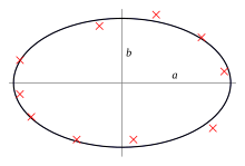
Conic fitting a set of points using least-squares approximation
The method of least squares is a standard approach in regression analysis to approximate the solution of overdetermined systems (sets of equations in which there are more equations than unknowns) by minimizing the sum of the squares of the residuals (a residual being the difference between an observed value and the fitted value provided by a model) made in the results of each individual equation.
The most important application is in data fitting. When the problem has substantial uncertainties in the independent variable (the x variable), then simple regression and least-squares methods have problems; in such cases, the methodology required for fitting errors-in-variables models may be considered instead of that for least squares.
Least squares problems fall into two categories: linear or ordinary least squares and nonlinear least squares, depending on whether or not the residuals are linear in all unknowns. The linear least-squares problem occurs in statistical regression analysis; it has a closed-form solution. The nonlinear problem is usually solved by iterative refinement; at each iteration the system is approximated by a linear one, and thus the core calculation is similar in both cases.
Polynomial least squares describes the variance in a prediction of the dependent variable as a function of the independent variable and the deviations from the fitted curve.
When the observations come from an exponential family with identity as its natural sufficient statistics and mild-conditions are satisfied (e.g. for normal, exponential, Poisson and binomial distributions), standardized least-squares estimates and maximum-likelihood estimates are identical.[1] The method of least squares can also be derived as a method of moments estimator.
The following discussion is mostly presented in terms of linear functions but the use of least squares is valid and practical for more general families of functions. Also, by iteratively applying local quadratic approximation to the likelihood (through the Fisher information), the least-squares method may be used to fit a generalized linear model.
The least-squares method was officially discovered and published by Adrien-Marie Legendre (1805),[2] though it is usually also co-credited to Carl Friedrich Gauss (1795)[3][4] who contributed significant theoretical advances to the method and may have previously used it in his work.[5][6]
History[edit]
Founding[edit]
The method of least squares grew out of the fields of astronomy and geodesy, as scientists and mathematicians sought to provide solutions to the challenges of navigating the Earth’s oceans during the Age of Discovery. The accurate description of the behavior of celestial bodies was the key to enabling ships to sail in open seas, where sailors could no longer rely on land sightings for navigation.
The method was the culmination of several advances that took place during the course of the eighteenth century:[7]
- The combination of different observations as being the best estimate of the true value; errors decrease with aggregation rather than increase, perhaps first expressed by Roger Cotes in 1722.
- The combination of different observations taken under the same conditions contrary to simply trying one’s best to observe and record a single observation accurately. The approach was known as the method of averages. This approach was notably used by Tobias Mayer while studying the librations of the moon in 1750, and by Pierre-Simon Laplace in his work in explaining the differences in motion of Jupiter and Saturn in 1788.
- The combination of different observations taken under different conditions. The method came to be known as the method of least absolute deviation. It was notably performed by Roger Joseph Boscovich in his work on the shape of the earth in 1757 and by Pierre-Simon Laplace for the same problem in 1799.
- The development of a criterion that can be evaluated to determine when the solution with the minimum error has been achieved. Laplace tried to specify a mathematical form of the probability density for the errors and define a method of estimation that minimizes the error of estimation. For this purpose, Laplace used a symmetric two-sided exponential distribution we now call Laplace distribution to model the error distribution, and used the sum of absolute deviation as error of estimation. He felt these to be the simplest assumptions he could make, and he had hoped to obtain the arithmetic mean as the best estimate. Instead, his estimator was the posterior median.
The method[edit]

The first clear and concise exposition of the method of least squares was published by Legendre in 1805.[8] The technique is described as an algebraic procedure for fitting linear equations to data and Legendre demonstrates the new method by analyzing the same data as Laplace for the shape of the earth. Within ten years after Legendre’s publication, the method of least squares had been adopted as a standard tool in astronomy and geodesy in France, Italy, and Prussia, which constitutes an extraordinarily rapid acceptance of a scientific technique.[7]
In 1809 Carl Friedrich Gauss published his method of calculating the orbits of celestial bodies. In that work he claimed to have been in possession of the method of least squares since 1795. This naturally led to a priority dispute with Legendre. However, to Gauss’s credit, he went beyond Legendre and succeeded in connecting the method of least squares with the principles of probability and to the normal distribution. He had managed to complete Laplace’s program of specifying a mathematical form of the probability density for the observations, depending on a finite number of unknown parameters, and define a method of estimation that minimizes the error of estimation. Gauss showed that the arithmetic mean is indeed the best estimate of the location parameter by changing both the probability density and the method of estimation. He then turned the problem around by asking what form the density should have and what method of estimation should be used to get the arithmetic mean as estimate of the location parameter. In this attempt, he invented the normal distribution.
An early demonstration of the strength of Gauss’s method came when it was used to predict the future location of the newly discovered asteroid Ceres. On 1 January 1801, the Italian astronomer Giuseppe Piazzi discovered Ceres and was able to track its path for 40 days before it was lost in the glare of the sun. Based on these data, astronomers desired to determine the location of Ceres after it emerged from behind the sun without solving Kepler’s complicated nonlinear equations of planetary motion. The only predictions that successfully allowed Hungarian astronomer Franz Xaver von Zach to relocate Ceres were those performed by the 24-year-old Gauss using least-squares analysis.
In 1810, after reading Gauss’s work, Laplace, after proving the central limit theorem, used it to give a large sample justification for the method of least squares and the normal distribution. In 1822, Gauss was able to state that the least-squares approach to regression analysis is optimal in the sense that in a linear model where the errors have a mean of zero, are uncorrelated, and have equal variances, the best linear unbiased estimator of the coefficients is the least-squares estimator. This result is known as the Gauss–Markov theorem.
The idea of least-squares analysis was also independently formulated by the American Robert Adrain in 1808. In the next two centuries workers in the theory of errors and in statistics found many different ways of implementing least squares.[9]
Problem statement[edit]
The objective consists of adjusting the parameters of a model function to best fit a data set. A simple data set consists of n points (data pairs)  , i = 1, …, n, where
  is an independent variable and
  is a dependent variable whose value is found by observation. The model function has the form
  , where m adjustable parameters are held in the vector
  . The goal is to find the parameter values for the model that «best» fits the data. The fit of a model to a data point is measured by its residual, defined as the difference between the observed value of the dependent variable and the value predicted by the model:


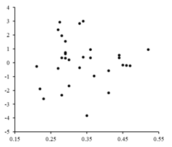
The residuals are plotted against corresponding
values. The random fluctuations about indicate a linear model is appropriate.

The least-squares method finds the optimal parameter values by minimizing the sum of squared residuals,  :[10]
:[10]

In the simplest case  and the result of the least-squares method is the arithmetic mean of the input data.
An example of a model in two dimensions is that of the straight line. Denoting the y-intercept as  and the slope as
  , the model function is given by
  . See linear least squares for a fully worked out example of this model.
A data point may consist of more than one independent variable. For example, when fitting a plane to a set of height measurements, the plane is a function of two independent variables, x and z, say. In the most general case there may be one or more independent variables and one or more dependent variables at each data point.
To the right is a residual plot illustrating random fluctuations about  , indicating that a linear model
 is appropriate.
  is an independent, random variable.[10]
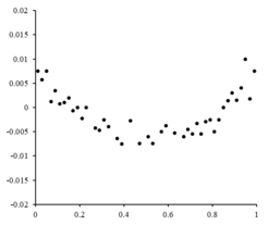
The residuals are plotted against the corresponding  values. The parabolic shape of the fluctuations about indicates a parabolic model is appropriate.
If the residual points had some sort of a shape and were not randomly fluctuating, a linear model would not be appropriate. For example, if the residual plot had a parabolic shape as seen to the right, a parabolic model  would be appropriate for the data. The residuals for a parabolic model can be calculated via
  .[10]
.[10]
Limitations[edit]
This regression formulation considers only observational errors in the dependent variable (but the alternative total least squares regression can account for errors in both variables). There are two rather different contexts with different implications:
- Regression for prediction. Here a model is fitted to provide a prediction rule for application in a similar situation to which the data used for fitting apply. Here the dependent variables corresponding to such future application would be subject to the same types of observation error as those in the data used for fitting. It is therefore logically consistent to use the least-squares prediction rule for such data.
- Regression for fitting a «true relationship». In standard regression analysis that leads to fitting by least squares there is an implicit assumption that errors in the independent variable are zero or strictly controlled so as to be negligible. When errors in the independent variable are non-negligible, models of measurement error can be used; such methods can lead to parameter estimates, hypothesis testing and confidence intervals that take into account the presence of observation errors in the independent variables.[11] An alternative approach is to fit a model by total least squares; this can be viewed as taking a pragmatic approach to balancing the effects of the different sources of error in formulating an objective function for use in model-fitting.
Solving the least squares problem[edit]
The minimum of the sum of squares is found by setting the gradient to zero. Since the model contains m parameters, there are m gradient equations:

and since  , the gradient equations become

The gradient equations apply to all least squares problems. Each particular problem requires particular expressions for the model and its partial derivatives.[12]
Linear least squares[edit]
A regression model is a linear one when the model comprises a linear combination of the parameters, i.e.,
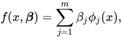
where the function  is a function of .[12]
Letting 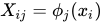 and putting the independent and dependent variables in matrices
  and
and  , respectively, we can compute the least squares in the following way. Note that
  is the set of all data.[12][13]

The gradient of the loss is:

Setting the gradient of the loss to zero and solving for , we get:[13][12]


Non-linear least squares[edit]
There is, in some cases, a closed-form solution to a non-linear least squares problem – but in general there is not. In the case of no closed-form solution, numerical algorithms are used to find the value of the parameters  that minimizes the objective. Most algorithms involve choosing initial values for the parameters. Then, the parameters are refined iteratively, that is, the values are obtained by successive approximation:

where a superscript k is an iteration number, and the vector of increments  is called the shift vector. In some commonly used algorithms, at each iteration the model may be linearized by approximation to a first-order Taylor series expansion about
  :
:
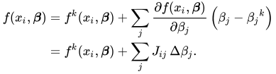
The Jacobian J is a function of constants, the independent variable and the parameters, so it changes from one iteration to the next. The residuals are given by

To minimize the sum of squares of  , the gradient equation is set to zero and solved for :

which, on rearrangement, become m simultaneous linear equations, the normal equations:

The normal equations are written in matrix notation as

These are the defining equations of the Gauss–Newton algorithm.
Differences between linear and nonlinear least squares[edit]
- The model function, f, in LLSQ (linear least squares) is a linear combination of parameters of the form The model may represent a straight line, a parabola or any other linear combination of functions. In NLLSQ (nonlinear least squares) the parameters appear as functions, such as and so forth. If the derivatives are either constant or depend only on the values of the independent variable, the model is linear in the parameters. Otherwise the model is nonlinear.
- Need initial values for the parameters to find the solution to a NLLSQ problem; LLSQ does not require them.
- Solution algorithms for NLLSQ often require that the Jacobian can be calculated similar to LLSQ. Analytical expressions for the partial derivatives can be complicated. If analytical expressions are impossible to obtain either the partial derivatives must be calculated by numerical approximation or an estimate must be made of the Jacobian, often via finite differences.
- Non-convergence (failure of the algorithm to find a minimum) is a common phenomenon in NLLSQ.
- LLSQ is globally concave so non-convergence is not an issue.
- Solving NLLSQ is usually an iterative process which has to be terminated when a convergence criterion is satisfied. LLSQ solutions can be computed using direct methods, although problems with large numbers of parameters are typically solved with iterative methods, such as the Gauss–Seidel method.
- In LLSQ the solution is unique, but in NLLSQ there may be multiple minima in the sum of squares.
- Under the condition that the errors are uncorrelated with the predictor variables, LLSQ yields unbiased estimates, but even under that condition NLLSQ estimates are generally biased.



These differences must be considered whenever the solution to a nonlinear least squares problem is being sought.[12]
Example[edit]
Consider a simple example drawn from physics. A spring should obey Hooke’s law which states that the extension of a spring y is proportional to the force, F, applied to it.

constitutes the model, where F is the independent variable. In order to estimate the force constant, k, we conduct a series of n measurements with different forces to produce a set of data,  , where yi is a measured spring extension.[14] Each experimental observation will contain some error,
  , and so we may specify an empirical model for our observations,

There are many methods we might use to estimate the unknown parameter k. Since the n equations in the m variables in our data comprise an overdetermined system with one unknown and n equations, we estimate k using least squares. The sum of squares to be minimized is
- [12]
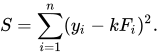
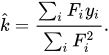
The least squares estimate of the force constant, k, is given by
We assume that applying force causes the spring to expand. After having derived the force constant by least squares fitting, we predict the extension from Hooke’s law.
Uncertainty quantification[edit]
In a least squares calculation with unit weights, or in linear regression, the variance on the jth parameter,
denoted  , is usually estimated with
![{displaystyle operatorname {var} ({hat {beta }}_{j})=sigma ^{2}left(left[X^{mathsf {T}}Xright]^{-1}right)_{jj}approx {hat {sigma }}^{2}C_{jj},}](https://wikimedia.org/api/rest_v1/media/math/render/svg/d85cf89d392a9c191ff1fe3429654bd748a02b2b)
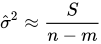
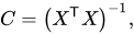
where the true error variance σ2 is replaced by an estimate, the reduced chi-squared statistic, based on the minimized value of the residual sum of squares (objective function), S. The denominator, n − m, is the statistical degrees of freedom; see effective degrees of freedom for generalizations.[12] C is the covariance matrix.
Statistical testing[edit]
If the probability distribution of the parameters is known or an asymptotic approximation is made, confidence limits can be found. Similarly, statistical tests on the residuals can be conducted if the probability distribution of the residuals is known or assumed. We can derive the probability distribution of any linear combination of the dependent variables if the probability distribution of experimental errors is known or assumed. Inferring is easy when assuming that the errors follow a normal distribution, consequently implying that the parameter estimates and residuals will also be normally distributed conditional on the values of the independent variables.[12]
It is necessary to make assumptions about the nature of the experimental errors to test the results statistically. A common assumption is that the errors belong to a normal distribution. The central limit theorem supports the idea that this is a good approximation in many cases.
- The Gauss–Markov theorem. In a linear model in which the errors have expectation zero conditional on the independent variables, are uncorrelated and have equal variances, the best linear unbiased estimator of any linear combination of the observations, is its least-squares estimator. «Best» means that the least squares estimators of the parameters have minimum variance. The assumption of equal variance is valid when the errors all belong to the same distribution.
- If the errors belong to a normal distribution, the least-squares estimators are also the maximum likelihood estimators in a linear model.
However, suppose the errors are not normally distributed. In that case, a central limit theorem often nonetheless implies that the parameter estimates will be approximately normally distributed so long as the sample is reasonably large. For this reason, given the important property that the error mean is independent of the independent variables, the distribution of the error term is not an important issue in regression analysis. Specifically, it is not typically important whether the error term follows a normal distribution.
Weighted least squares[edit]

«Fanning Out» Effect of Heteroscedasticity
A special case of generalized least squares called weighted least squares occurs when all the off-diagonal entries of Ω (the correlation matrix of the residuals) are null; the variances of the observations (along the covariance matrix diagonal) may still be unequal (heteroscedasticity). In simpler terms, heteroscedasticity is when the variance of  depends on the value of
  which causes the residual plot to create a «fanning out» effect towards larger values as seen in the residual plot to the right. On the other hand, homoscedasticity is assuming that the variance of and variance of are equal.[10]
Relationship to principal components[edit]
The first principal component about the mean of a set of points can be represented by that line which most closely approaches the data points (as measured by squared distance of closest approach, i.e. perpendicular to the line). In contrast, linear least squares tries to minimize the distance in the  direction only. Thus, although the two use a similar error metric, linear least squares is a method that treats one dimension of the data preferentially, while PCA treats all dimensions equally.
Relationship to measure theory[edit]
Notable statistician Sara van de Geer used empirical process theory and the Vapnik–Chervonenkis dimension to prove a least-squares estimator can be interpreted as a measure on the space of square-integrable functions.[15]
Regularization[edit]
Tikhonov regularization[edit]
In some contexts a regularized version of the least squares solution may be preferable. Tikhonov regularization (or ridge regression) adds a constraint that  , the squared
  -norm of the parameter vector, is not greater than a given value to the least squares formulation, leading to a constrained minimization problem. This is equivalent to the unconstrained minimization problem where the objective function is the residual sum of squares plus a penalty term
  and
and  is a tuning parameter (this is the Lagrangian form of the constrained minimization problem).[16]
In a Bayesian context, this is equivalent to placing a zero-mean normally distributed prior on the parameter vector.
Lasso method[edit]
An alternative regularized version of least squares is Lasso (least absolute shrinkage and selection operator), which uses the constraint that  , the L1-norm of the parameter vector, is no greater than a given value.[17][18][19] (One can show like above using Lagrange multipliers that this is equivalent to an unconstrained minimization of the least-squares penalty with
  added.) In a Bayesian context, this is equivalent to placing a zero-mean Laplace prior distribution on the parameter vector.[20] The optimization problem may be solved using quadratic programming or more general convex optimization methods, as well as by specific algorithms such as the least angle regression algorithm.
One of the prime differences between Lasso and ridge regression is that in ridge regression, as the penalty is increased, all parameters are reduced while still remaining non-zero, while in Lasso, increasing the penalty will cause more and more of the parameters to be driven to zero. This is an advantage of Lasso over ridge regression, as driving parameters to zero deselects the features from the regression. Thus, Lasso automatically selects more relevant features and discards the others, whereas Ridge regression never fully discards any features. Some feature selection techniques are developed based on the LASSO including Bolasso which bootstraps samples,[21] and FeaLect which analyzes the regression coefficients corresponding to different values of to score all the features.[22]
The L1-regularized formulation is useful in some contexts due to its tendency to prefer solutions where more parameters are zero, which gives solutions that depend on fewer variables.[17] For this reason, the Lasso and its variants are fundamental to the field of compressed sensing. An extension of this approach is elastic net regularization.
See also[edit]
- Least-squares adjustment
- Bayesian MMSE estimator
- Best linear unbiased estimator (BLUE)
- Best linear unbiased prediction (BLUP)
- Gauss–Markov theorem
- L2 norm
- Least absolute deviations
- Least-squares spectral analysis
- Measurement uncertainty
- Orthogonal projection
- Proximal gradient methods for learning
- Quadratic loss function
- Root mean square
- Squared deviations from the mean
References[edit]
- ^ Charnes, A.; Frome, E. L.; Yu, P. L. (1976). «The Equivalence of Generalized Least Squares and Maximum Likelihood Estimates in the Exponential Family». Journal of the American Statistical Association. 71 (353): 169–171. doi:10.1080/01621459.1976.10481508.
- ^ Mansfield Merriman, «A List of Writings Relating to the Method of Least Squares»
- ^ Bretscher, Otto (1995). Linear Algebra With Applications (3rd ed.). Upper Saddle River, NJ: Prentice Hall.
- ^ Stigler, Stephen M. (1981). «Gauss and the Invention of Least Squares». Ann. Stat. 9 (3): 465–474. doi:10.1214/aos/1176345451.
- ^ Britannica, «Least squares method»
- ^ Studies in the History of Probability and Statistics. XXIX: The Discovery of the Method of Least Squares
R. L. Plackett - ^ a b Stigler, Stephen M. (1986). The History of Statistics: The Measurement of Uncertainty Before 1900. Cambridge, MA: Belknap Press of Harvard University Press. ISBN 978-0-674-40340-6.
- ^ Legendre, Adrien-Marie (1805), Nouvelles méthodes pour la détermination des orbites des comètes [New Methods for the Determination of the Orbits of Comets] (in French), Paris: F. Didot, hdl:2027/nyp.33433069112559
- ^ Aldrich, J. (1998). «Doing Least Squares: Perspectives from Gauss and Yule». International Statistical Review. 66 (1): 61–81. doi:10.1111/j.1751-5823.1998.tb00406.x. S2CID 121471194.
- ^ a b c d A modern introduction to probability and statistics: understanding why and how. Dekking, Michel, 1946-. London: Springer. 2005. ISBN 978-1-85233-896-1. OCLC 262680588.
{{cite book}}: CS1 maint: others (link) - ^ For a good introduction to error-in-variables, please see Fuller, W. A. (1987). Measurement Error Models. John Wiley & Sons. ISBN 978-0-471-86187-4.
- ^ a b c d e f g h Williams, Jeffrey H. (Jeffrey Huw), 1956- (November 2016). Quantifying measurement: the tyranny of numbers. Morgan & Claypool Publishers, Institute of Physics (Great Britain). San Rafael [California] (40 Oak Drive, San Rafael, CA, 94903, USA). ISBN 978-1-68174-433-9. OCLC 962422324.
{{cite book}}: CS1 maint: location (link) CS1 maint: multiple names: authors list (link) - ^ a b Rencher, Alvin C.; Christensen, William F. (2012-08-15). Methods of Multivariate Analysis. John Wiley & Sons. p. 155. ISBN 978-1-118-39167-9.
- ^ Gere, James M. (2013). Mechanics of materials. Goodno, Barry J. (8th ed.). Stamford, Conn.: Cengage Learning. ISBN 978-1-111-57773-5. OCLC 741541348.
- ^ van de Geer, Sara (June 1987). «A New Approach to Least-Squares Estimation, with Applications». Annals of Statistics. 15 (2): 587–602. doi:10.1214/aos/1176350362. S2CID 123088844.
- ^ van Wieringen, Wessel N. (2021). «Lecture notes on ridge regression» (PDF). arXiv:1509.09169.
- ^ a b Tibshirani, R. (1996). «Regression shrinkage and selection via the lasso». Journal of the Royal Statistical Society, Series B. 58 (1): 267–288. JSTOR 2346178.
- ^ Hastie, Trevor; Tibshirani, Robert; Friedman, Jerome H. (2009). The Elements of Statistical Learning (second ed.). Springer-Verlag. ISBN 978-0-387-84858-7. Archived from the original on 2009-11-10.
- ^ Bühlmann, Peter; van de Geer, Sara (2011). Statistics for High-Dimensional Data: Methods, Theory and Applications. Springer. ISBN 9783642201929.
- ^ Park, Trevor; Casella, George (2008). «The Bayesian Lasso». Journal of the American Statistical Association. 103 (482): 681–686. doi:10.1198/016214508000000337. S2CID 11797924.
- ^ Bach, Francis R (2008). «Bolasso: model consistent lasso estimation through the bootstrap». Proceedings of the 25th International Conference on Machine Learning. Icml ’08: 33–40. arXiv:0804.1302. Bibcode:2008arXiv0804.1302B. doi:10.1145/1390156.1390161. ISBN 9781605582054. S2CID 609778.
- ^ Zare, Habil (2013). «Scoring relevancy of features based on combinatorial analysis of Lasso with application to lymphoma diagnosis». BMC Genomics. 14 (Suppl 1): S14. doi:10.1186/1471-2164-14-S1-S14. PMC 3549810. PMID 23369194.
Further reading[edit]
- Björck, Å. (1996). Numerical Methods for Least Squares Problems. SIAM. ISBN 978-0-89871-360-2.
- Kariya, T.; Kurata, H. (2004). Generalized Least Squares. Hoboken: Wiley. ISBN 978-0-470-86697-9.
- Luenberger, D. G. (1997) [1969]. «Least-Squares Estimation». Optimization by Vector Space Methods. New York: John Wiley & Sons. pp. 78–102. ISBN 978-0-471-18117-0.
- Rao, C. R.; Toutenburg, H.; et al. (2008). Linear Models: Least Squares and Alternatives. Springer Series in Statistics (3rd ed.). Berlin: Springer. ISBN 978-3-540-74226-5.
- Van de moortel, Koen (April 2021). «Multidirectional regression analysis».
- Wolberg, J. (2005). Data Analysis Using the Method of Least Squares: Extracting the Most Information from Experiments. Berlin: Springer. ISBN 978-3-540-25674-8.
External links[edit]
 Media related to Least squares at Wikimedia Commons
 Media related to Least squares at Wikimedia Commons
With Machine Learning and Artificial Intelligence booming the IT market it has become essential to learn the fundamentals of these trending technologies. This blog on Least Squares Regression Method will help you understand the math behind Regression Analysis and how it can be implemented using Python.
To get in-depth knowledge of Artificial Intelligence and Machine Learning, you can enroll for live Machine Learning Engineer Master Program by Edureka with 24/7 support and lifetime access.
Here’s a list of topics that will be covered in this blog:
- What Is the Least Squares Method?
- Line Of Best Fit
- Steps to Compute the Line Of Best Fit
- The least-squares regression method with an example
- A short python script to implement Linear Regression
What is the Least Squares Regression Method?
The least-squares regression method is a technique commonly used in Regression Analysis. It is a mathematical method used to find the best fit line that represents the relationship between an independent and dependent variable.
To understand the least-squares regression method lets get familiar with the concepts involved in formulating the line of best fit.
What is the Line Of Best Fit?
Line of best fit is drawn to represent the relationship between 2 or more variables. To be more specific, the best fit line is drawn across a scatter plot of data points in order to represent a relationship between those data points.
Regression analysis makes use of mathematical methods such as least squares to obtain a definite relationship between the predictor variable (s) and the target variable. The least-squares method is one of the most effective ways used to draw the line of best fit. It is based on the idea that the square of the errors obtained must be minimized to the most possible extent and hence the name least squares method.
If we were to plot the best fit line that shows the depicts the sales of a company over a period of time, it would look something like this:
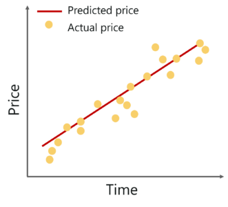
Notice that the line is as close as possible to all the scattered data points. This is what an ideal best fit line looks like.
To better understand the whole process let’s see how to calculate the line using the Least Squares Regression.
Steps to calculate the Line of Best Fit
To start constructing the line that best depicts the relationship between variables in the data, we first need to get our basics right. Take a look at the equation below:

Surely, you’ve come across this equation before. It is a simple equation that represents a straight line along 2 Dimensional data, i.e. x-axis and y-axis. To better understand this, let’s break down the equation:
- y: dependent variable
- m: the slope of the line
- x: independent variable
- c: y-intercept
So the aim is to calculate the values of slope, y-intercept and substitute the corresponding ‘x’ values in the equation in order to derive the value of the dependent variable.
Let’s see how this can be done.
As an assumption, let’s consider that there are ‘n’ data points.
Step 1: Calculate the slope ‘m’ by using the following formula:

Step 2: Compute the y-intercept (the value of y at the point where the line crosses the y-axis):

Step 3: Substitute the values in the final equation:

Simple, isn’t it?
Now let’s look at an example and see how you can use the least-squares regression method to compute the line of best fit.
Consider an example. Tom who is the owner of a retail shop, found the price of different T-shirts vs the number of T-shirts sold at his shop over a period of one week.
He tabulated this like shown below:
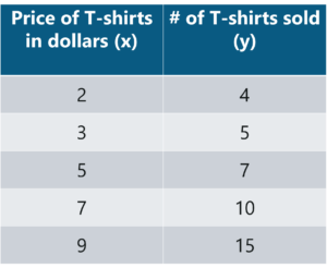
Let us use the concept of least squares regression to find the line of best fit for the above data.
Step 1: Calculate the slope ‘m’ by using the following formula:
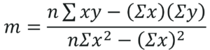
After you substitute the respective values, m = 1.518 approximately.
Step 2: Compute the y-intercept value

After you substitute the respective values, c = 0.305 approximately.
Step 3: Substitute the values in the final equation

Once you substitute the values, it should look something like this:

Let’s construct a graph that represents the y=mx + c line of best fit:
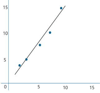
Now Tom can use the above equation to estimate how many T-shirts of price $8 can he sell at the retail shop.
y = 1.518 x 8 + 0.305 = 12.45 T-shirts
This comes down to 13 T-shirts! That’s how simple it is to make predictions using Linear Regression.
Now let’s try to understand based on what factors can we confirm that the above line is the line of best fit.
The least squares regression method works by minimizing the sum of the square of the errors as small as possible, hence the name least squares. Basically the distance between the line of best fit and the error must be minimized as much as possible. This is the basic idea behind the least squares regression method.
A few things to keep in mind before implementing the least squares regression method is:
- The data must be free of outliers because they might lead to a biased and wrongful line of best fit.
- The line of best fit can be drawn iteratively until you get a line with the minimum possible squares of errors.
- This method works well even with non-linear data.
- Technically, the difference between the actual value of ‘y’ and the predicted value of ‘y’ is called the Residual (denotes the error).
Now let’s wrap up by looking at a practical implementation of linear regression using Python.
Least Squares Regression In Python
In this section, we will be running a simple demo to understand the working of Regression Analysis using the least squares regression method. A short disclaimer, I’ll be using Python for this demo, if you’re not familiar with the language, you can go through the following blogs:
- Python Tutorial – A Complete Guide to Learn Python Programming
- Python Programming Language – Headstart With Python Basics
- A Beginners Guide To Python Functions
- Python for Data Science
Problem Statement: To apply Linear Regression and build a model that studies the relationship between the head size and the brain weight of an individual.
Data Set Description: The data set contains the following variables:
- Gender: Male or female represented as binary variables
- Age: Age of an individual
- Head size in cm^3: An individuals head size in cm^3
- Brain weight in grams: The weight of an individual’s brain measured in grams
These variables need to be analyzed in order to build a model that studies the relationship between the head size and brain weight of an individual.
Logic: To implement Linear Regression in order to build a model that studies the relationship between an independent and dependent variable. The model will be evaluated by using least square regression method where RMSE and R-squared will be the model evaluation parameters.
Let’s get started!
Step 1: Import the required libraries
import numpy as np
import pandas as pd
import matplotlib.pyplot as plt
Step 2: Import the data set
# Reading Data
data = pd.read_csv('C:UsersNeelTempDesktopheadbrain.csv')
print(data.shape)
(237, 4)
print(data.head())
   Gender  Age Range  Head Size(cm^3)  Brain Weight(grams)
0       1          1             4512                 1530
1       1          1             3738                 1297
2       1          1             4261                 1335
3       1          1             3777                 1282
4       1          1             4177                 1590
Step 3: Assigning ‘X’ as independent variable and ‘Y’ as dependent variable
# Coomputing X and Y
X = data['Head Size(cm^3)'].values
Y = data['Brain Weight(grams)'].values
Next, in order to calculate the slope and y-intercept we first need to compute the means of ‘x’ and ‘y’. This can be done as shown below:
# Mean X and Y
mean_x = np.mean(X)
mean_y = np.mean(Y)

# Total number of values
n = len(X)
Step 4: Calculate the values of the slope and y-intercept
# Using the formula to calculate 'm' and 'c'
numer = 0
denom = 0
for i in range(n):
numer += (X[i] - mean_x) * (Y[i] - mean_y)
denom += (X[i] - mean_x) ** 2
m = numer / denom
c = mean_y - (m * mean_x)

# Printing coefficients
print("Coefficients")
print(m, c)

Coefficients
0.26342933948939945 325.57342104944223
The above coefficients are our slope and intercept values respectively. On substituting the values in the final equation, we get:
Brain Weight = 325.573421049 + 0.263429339489 * Head Size
As simple as that, the above equation represents our linear model.
Now let’s plot this graphically.
Step 5: Plotting the line of best fit
# Plotting Values and Regression Line

max_x = np.max(X) + 100
min_x = np.min(X) - 100

# Calculating line values x and y
x = np.linspace(min_x, max_x, 1000)
y = c + m * x

# Ploting Line
plt.plot(x, y, color='#58b970', label='Regression Line')
# Ploting Scatter Points
plt.scatter(X, Y, c='#ef5423', label='Scatter Plot')

plt.xlabel('Head Size in cm3')
plt.ylabel('Brain Weight in grams')
plt.legend()
plt.show()

Step 6: Model Evaluation
The model built is quite good given the fact that our data set is of a small size. It’s time to evaluate the model and see how good it is for the final stage i.e., prediction. To do that we will use the Root Mean Squared Error method that basically calculates the least-squares error and takes a root of the summed values.
Mathematically speaking, Root Mean Squared Error is nothing but the square root of the sum of all errors divided by the total number of values. This is the formula to calculate RMSE:
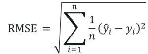
In the above equation, is the ith predicted output value. Let’s see how this can be done using Python.
# Calculating Root Mean Squares Error
rmse = 0
for i in range(n):
    y_pred = c + m * X[i]
    rmse += (Y[i] - y_pred) ** 2
rmse = np.sqrt(rmse/n)
print("RMSE")
print(rmse)
RMSE
72.1206213783709
Another model evaluation parameter is the statistical method called, R-squared value that measures how close the data are to the fitted line of best
fit.
Mathematically, it can be calculated as:
- is the total sum of squares
- is the total sum of squares of residuals
The value of R-squared ranges between 0 and 1. A negative value denoted that the model is weak and the prediction thus made are wrong and biased. In such situations, it’s essential that you analyze all the predictor variables and look for a variable that has a high correlation with the output. This step usually falls under EDA or Exploratory Data Analysis.
Let’s not get carried away. Here’s how you implement the computation of R-squared in Python:
# Calculating R2 Score
ss_tot = 0
ss_res = 0
for i in range(n):
    y_pred = c + m * X[i]
    ss_tot += (Y[i] - mean_y) ** 2
    ss_res += (Y[i] - y_pred) ** 2
r2 = 1 - (ss_res/ss_tot)
print("R2 Score")
print(r2)
R2 Score
0.6393117199570003
As you can see our R-squared value is quite close to 1, this denotes that our model is doing good and can be used for further predictions.
So that was the entire implementation of Least Squares Regression method using Python. Now that you know the math behind Regression Analysis, I’m sure you’re curious to learn more. Here are a few blogs to get you started:
- A Complete Guide To Maths And Statistics For Data Science
- All You Need To Know About Statistics And Probability
- Introduction To Markov Chains With Examples – Markov Chains With Python
- How To Implement Bayesian Networks In Python? – Bayesian Networks Explained With Examples
With this, we come to the end of this blog. If you have any queries regarding this topic, please leave a comment below and we’ll get back to you.
If you wish to enroll for a complete course on Artificial Intelligence and Machine Learning, Edureka has a specially curated Machine Learning Engineer Master Program that will make you proficient in techniques like Supervised Learning, Unsupervised Learning, and Natural Language Processing. It includes training on the latest advancements and technical approaches in Artificial Intelligence & Machine Learning such as Deep Learning, Graphical Models and Reinforcement Learning.
15.3. The Method of Least Squares#
We have developed the equation of the regression line that runs through a football shaped scatter plot. But not all scatter plots are football shaped, not even linear ones. Does every scatter plot have a “best” line that goes through it? If so, can we still use the formulas for the slope and intercept developed in the previous section, or do we need new ones?
To address these questions, we need a reasonable definition of “best”. Recall that the purpose of the line is to predict or estimate values of (y), given values of (x). Estimates typically aren’t perfect. Each one is off the true value by an error. A reasonable criterion for a line to be the “best” is for it to have the smallest possible overall error among all straight lines.
In this section we will make this criterion precise and see if we can identify the best straight line under the criterion.
Our first example is a dataset that has one row for every chapter of the novel “Little Women.” The goal is to estimate the number of characters (that is, letters, spaces punctuation marks, and so on) based on the number of periods. Recall that we attempted to do this in the very first lecture of this course.
little_women = Table.read_table(path_data + 'little_women.csv')
little_women = little_women.move_to_start('Periods')
little_women.show(3)
| Periods | Characters |
|---|---|
| 189 | 21759 |
| 188 | 22148 |
| 231 | 20558 |
… (44 rows omitted)
little_women.scatter('Periods', 'Characters')

To explore the data, we will need to use the functions correlation, slope, intercept, and fit defined in the previous section.
correlation(little_women, 'Periods', 'Characters')
The scatter plot is remarkably close to linear, and the correlation is more than 0.92.
15.3.1. Error in Estimation#
The graph below shows the scatter plot and line that we developed in the previous section. We don’t yet know if that’s the best among all lines. We first have to say precisely what “best” means.
lw_with_predictions = little_women.with_column('Linear Prediction', fit(little_women, 'Periods', 'Characters'))
lw_with_predictions.scatter('Periods')

Corresponding to each point on the scatter plot, there is an error of prediction calculated as the actual value minus the predicted value. It is the vertical distance between the point and the line, with a negative sign if the point is below the line.
actual = lw_with_predictions.column('Characters')
predicted = lw_with_predictions.column('Linear Prediction')
errors = actual - predicted
lw_with_predictions.with_column('Error', errors)
| Periods | Characters | Linear Prediction | Error |
|---|---|---|---|
| 189 | 21759 | 21183.6 | 575.403 |
| 188 | 22148 | 21096.6 | 1051.38 |
| 231 | 20558 | 24836.7 | -4278.67 |
| 195 | 25526 | 21705.5 | 3820.54 |
| 255 | 23395 | 26924.1 | -3529.13 |
| 140 | 14622 | 16921.7 | -2299.68 |
| 131 | 14431 | 16138.9 | -1707.88 |
| 214 | 22476 | 23358 | -882.043 |
| 337 | 33767 | 34056.3 | -289.317 |
| 185 | 18508 | 20835.7 | -2327.69 |
… (37 rows omitted)
We can use slope and intercept to calculate the slope and intercept of the fitted line. The graph below shows the line (in light blue). The errors corresponding to four of the points are shown in red. There is nothing special about those four points. They were just chosen for clarity of the display. The function lw_errors takes a slope and an intercept (in that order) as its arguments and draws the figure.
lw_reg_slope = slope(little_women, 'Periods', 'Characters')
lw_reg_intercept = intercept(little_women, 'Periods', 'Characters')
print('Slope of Regression Line:    ', np.round(lw_reg_slope), 'characters per period')
print('Intercept of Regression Line:', np.round(lw_reg_intercept), 'characters')
lw_errors(lw_reg_slope, lw_reg_intercept)
Slope of Regression Line:     87.0 characters per period
Intercept of Regression Line: 4745.0 characters

Had we used a different line to create our estimates, the errors would have been different. The graph below shows how big the errors would be if we were to use another line for estimation. The second graph shows large errors obtained by using a line that is downright silly.


15.3.2. Root Mean Squared Error#
What we need now is one overall measure of the rough size of the errors. You will recognize the approach to creating this – it’s exactly the way we developed the SD.
If you use any arbitrary line to calculate your estimates, then some of your errors are likely to be positive and others negative. To avoid cancellation when measuring the rough size of the errors, we will take the mean of the squared errors rather than the mean of the errors themselves.
The mean squared error of estimation is a measure of roughly how big the squared errors are, but as we have noted earlier, its units are hard to interpret. Taking the square root yields the root mean square error (rmse), which is in the same units as the variable being predicted and therefore much easier to understand.
15.3.3. Minimizing the Root Mean Squared Error#
Our observations so far can be summarized as follows.
-
To get estimates of (y) based on (x), you can use any line you want.
-
Every line has a root mean squared error of estimation.
-
“Better” lines have smaller errors.
Is there a “best” line? That is, is there a line that minimizes the root mean squared error among all lines?
To answer this question, we will start by defining a function lw_rmse to compute the root mean squared error of any line through the Little Women scatter diagram. The function takes the slope and the intercept (in that order) as its arguments.
def lw_rmse(slope, intercept):
    lw_errors(slope, intercept)
    x = little_women.column('Periods')
    y = little_women.column('Characters')
    fitted = slope * x + intercept
    mse = np.mean((y - fitted) ** 2)
    print("Root mean squared error:", mse ** 0.5)
Root mean squared error: 4322.167831766537

Root mean squared error: 16710.11983735375

Bad lines have big values of rmse, as expected. But the rmse is much smaller if we choose a slope and intercept close to those of the regression line.
Root mean squared error: 2715.5391063834586

Here is the root mean squared error corresponding to the regression line. By a remarkable fact of mathematics, no other line can beat this one.
-
The regression line is the unique straight line that minimizes the mean squared error of estimation among all straight lines.
lw_rmse(lw_reg_slope, lw_reg_intercept)
Root mean squared error: 2701.690785311856

The proof of this statement requires abstract mathematics that is beyond the scope of this course. On the other hand, we do have a powerful tool – Python – that performs large numerical computations with ease. So we can use Python to confirm that the regression line minimizes the mean squared error.
15.3.3.1. Numerical Optimization#
First note that a line that minimizes the root mean squared error is also a line that minimizes the squared error. The square root makes no difference to the minimization. So we will save ourselves a step of computation and just minimize the mean squared error (mse).
We are trying to predict the number of characters ((y)) based on the number of periods ((x)) in chapters of Little Women. If we use the line
[
mbox{prediction} ~=~ ax + b
]
it will have an mse that depends on the slope (a) and the intercept (b). The function lw_mse takes the slope and intercept as its arguments and returns the corresponding mse.
def lw_mse(any_slope, any_intercept):
    x = little_women.column('Periods')
    y = little_women.column('Characters')
    fitted = any_slope*x + any_intercept
    return np.mean((y - fitted) ** 2)
Let’s check that lw_mse gets the right answer for the root mean squared error of the regression line. Remember that lw_mse returns the mean squared error, so we have to take the square root to get the rmse.
lw_mse(lw_reg_slope, lw_reg_intercept)**0.5
That’s the same as the value we got by using lw_rmse earlier:
lw_rmse(lw_reg_slope, lw_reg_intercept)
Root mean squared error: 2701.690785311856

You can confirm that lw_mse returns the correct value for other slopes and intercepts too. For example, here is the rmse of the extremely bad line that we tried earlier.
And here is the rmse for a line that is close to the regression line.
If we experiment with different values, we can find a low-error slope and intercept through trial and error, but that would take a while. Fortunately, there is a Python function that does all the trial and error for us.
The minimize function can be used to find the arguments of a function for which the function returns its minimum value. Python uses a similar trial-and-error approach, following the changes that lead to incrementally lower output values.
The argument of minimize is a function that itself takes numerical arguments and returns a numerical value. For example, the function lw_mse takes a numerical slope and intercept as its arguments and returns the corresponding mse.
The call minimize(lw_mse) returns an array consisting of the slope and the intercept that minimize the mse. These minimizing values are excellent approximations arrived at by intelligent trial-and-error, not exact values based on formulas.
best = minimize(lw_mse)
best
array([ 86.97784117, 4744.78484535])
These values are the same as the values we calculated earlier by using the slope and intercept functions. We see small deviations due to the inexact nature of minimize, but the values are essentially the same.
print("slope from formula:        ", lw_reg_slope)
print("slope from minimize:       ", best.item(0))
print("intercept from formula:    ", lw_reg_intercept)
print("intercept from minimize:   ", best.item(1))
slope from formula:         86.97784125829821
slope from minimize:        86.97784116615884
intercept from formula:     4744.784796574928
intercept from minimize:    4744.784845352655
15.3.4. The Least Squares Line#
Therefore, we have found not only that the regression line minimizes mean squared error, but also that minimizing mean squared error gives us the regression line. The regression line is the only line that minimizes mean squared error.
That is why the regression line is sometimes called the “least squares line.”
Least square method is the process of finding a regression line or best-fitted line for any data set that is described by an equation. This method requires reducing the sum of the squares of the residual parts of the points from the curve or line and the trend of outcomes is found quantitatively. The method of curve fitting is seen while regression analysis and the fitting equations to derive the curve is the least square method.
Let us look at a simple example, Ms. Dolma said in the class «Hey students who spend more time on their assignments are getting better grades». A student wants to estimate his grade for spending 2.3 hours on an assignment. Through the magic of the least-squares method, it is possible to determine the predictive model that will help him estimate the grades far more accurately. This method is much simpler because it requires nothing more than some data and maybe a calculator.
In this section, we’re going to explore least squares, understand what it means, learn the general formula, steps to plot it on a graph, know what are its limitations, and see what tricks we can use with least squares.
| 1. | Least Square Method Definition |
| 2. | Limitations for Least Square Method |
| 3. | Least Square Method Graph |
| 4. | Least Square Method Formula |
| 5. | FAQs on Least Square Method |
Least Square Method Definition
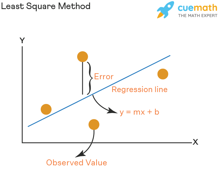
The least-squares method is a statistical method used to find the line of best fit of the form of an equation such as y = mx + b to the given data. The curve of the equation is called the regression line. Our main objective in this method is to reduce the sum of the squares of errors as much as possible. This is the reason this method is called the least-squares method. This method is often used in data fitting where the best fit result is assumed to reduce the sum of squared errors that is considered to be the difference between the observed values and corresponding fitted value. The sum of squared errors helps in finding the variation in observed data. For example, we have 4 data points and using this method we arrive at the following graph.
The two basic categories of least-square problems are ordinary or linear least squares and nonlinear least squares.
Limitations for Least Square Method
Even though the least-squares method is considered the best method to find the line of best fit, it has a few limitations. They are:
- This method exhibits only the relationship between the two variables. All other causes and effects are not taken into consideration.
- This method is unreliable when data is not evenly distributed.
- This method is very sensitive to outliers. In fact, this can skew the results of the least-squares analysis.
Least Square Method Graph
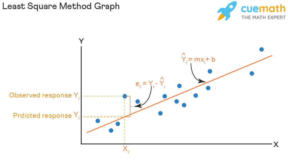
Look at the graph below, the straight line shows the potential relationship between the independent variable and the dependent variable. The ultimate goal of this method is to reduce this difference between the observed response and the response predicted by the regression line. Less residual means that the model fits better. The data points need to be minimized by the method of reducing residuals of each point from the line. There are vertical residuals and perpendicular residuals. Vertical is mostly used in polynomials and hyperplane problems while perpendicular is used in general as seen in the image below.
Least Square Method Formula
Least-square method is the curve that best fits a set of observations with a minimum sum of squared residuals or errors. Let us assume that the given points of data are (x1, y1), (x2, y2), (x3, y3), …, (xn, yn) in which all x’s are independent variables, while all y’s are dependent ones. This method is used to find a linear line of the form y = mx + b, where y and x are variables, m is the slope, and b is the y-intercept. The formula to calculate slope m and the value of b is given by:
m = (n∑xy — ∑y∑x)/n∑x2 — (∑x)2
b = (∑y — m∑x)/n
Here, n is the number of data points.
Following are the steps to calculate the least square using the above formulas.
- Step 1: Draw a table with 4 columns where the first two columns are for x and y points.
- Step 2: In the next two columns, find xy and (x)2.
- Step 3: Find ∑x, ∑y, ∑xy, and ∑(x)2.
- Step 4: Find the value of slope m using the above formula.
- Step 5: Calculate the value of b using the above formula.
- Step 6: Substitute the value of m and b in the equation y = mx + b
Let us look at an example to understand this better.
Example: Let’s say we have data as shown below.
| x | 1 | 2 | 3 | 4 | 5 |
|---|---|---|---|---|---|
| y | 2 | 5 | 3 | 8 | 7 |
Solution: We will follow the steps to find the linear line.
| x | y | xy | x2 |
|---|---|---|---|
| 1 | 2 | 2 | 1 |
| 2 | 5 | 10 | 4 |
| 3 | 3 | 9 | 9 |
| 4 | 8 | 32 | 16 |
| 5 | 7 | 35 | 25 |
| ∑x =15 | ∑y = 25 | ∑xy = 88 | ∑x2 = 55 |
Find the value of m by using the formula,
m = (n∑xy — ∑y∑x)/n∑x2 — (∑x)2
m = [(5×88) — (15×25)]/(5×55) — (15)2
m = (440 — 375)/(275 — 225)
m = 65/50 = 13/10
Find the value of b by using the formula,
b = (∑y — m∑x)/n
b = (25 — 1.3×15)/5
b = (25 — 19.5)/5
b = 5.5/5
So, the required equation of least squares is y = mx + b = 13/10x + 5.5/5.
Important Notes
- The least-squares method is used to predict the behavior of the dependent variable with respect to the independent variable.
- The sum of the squares of errors is called variance.
- The main aim of the least-squares method is to minimize the sum of the squared errors.
Related Topics
Listed below are a few topics related to least-square method.
- Parabola
- Hyperbola
- x and y graph
- Slope
FAQs on Least Square Method
What are Ordinary Least Squares Used For?
The ordinary least squares method is used to find the predictive model that best fits our data points.
Is Least Squares the Same as Linear Regression?
No, linear regression and least-squares are not the same. Linear regression is the analysis of statistical data to predict the value of the quantitative variable. Least squares is one of the methods used in linear regression to find the predictive model.
How do Outliers Affect the Least-Squares Regression Line?
The presence of unusual data points can skew the results of the linear regression. This makes the validity of the model very critical to obtain sound answers to the questions motivating the formation of the predictive model.
What is Least Square Method Formula?
For determining the equation of line for any data, we need to use the equation y = mx + b. The least-square method formula is by finding the value of both m and b by using the formulas:
m = (n∑xy — ∑y∑x)/n∑x2 — (∑x)2
b = (∑y — m∑x)/n
Here, n is the number of data points.
What is Least Square Method in Regression?
The least-square regression helps in calculating the best fit line of the set of data from both the activity levels and corresponding total costs. The idea behind the calculation is to minimize the sum of the squares of the vertical errors between the data points and cost function.
Why Least Square Method is Used?
Least squares is used as an equivalent to maximum likelihood when the model residuals are normally distributed with mean of 0.
What is Least Square Curve Fitting?
Least square method is the process of fitting a curve according to the given data. It is one of the methods used to determine the trend line for the given data.
Key focus: Understand step by step, the least squares estimator for parameter estimation. Hands-on example to fit a curve using least squares estimation
Background:
The various estimation concepts/techniques like Maximum Likelihood Estimation (MLE), Minimum Variance Unbiased Estimation (MVUE), Best Linear Unbiased Estimator (BLUE) – all falling under the umbrella of classical estimation – require assumptions/knowledge on second order statistics (covariance) before the estimation technique can be applied. Linear estimators, discussed here, do not require any statistical model to begin with. It only requires a signal model in linear form.
Linear models are ubiquitously used in various fields for studying the relationship between two or more variables. Linear models include regression analysis models, ANalysis Of VAriance (ANOVA) models, variance component models etc. Here, one variable is considered as a dependent (response) variable which can be expressed as a linear combination of one or more independent (explanatory) variables.
Studying the dependence between variables is fundamental to linear models. For applying the concepts to real application, following procedure is required
- Problem identification
- Model selection
- Statistical performance analysis
- Criticism of the model based on statistical analysis
- Conclusions and recommendations
Following text seeks to elaborate on linear models when applied to parameter estimation using Ordinary Least Squares (OLS).
Linear Regression Model
A regression model relates a dependent (response) variable y to a set of k independent explanatory variables {x1, x2 ,…, xk} using a function. When the relationship is not exact, an error term e is introduced.

If the function f is not a linear function, the above model is referred as Non-Linear Regression Model. If f is linear, equation (1) is expressed as linear combination of independent variables xk weighted by unknown vector parameters θ = {θ1, θ2,…, θk } that we wish to estimate.

Equation (2) is referred as Linear Regression model. When N such observations are made

where,
yi – response variable
xi – independent variables – known expressed as observed matrix X with rank k
θi – set of parameters to be estimated
e – disturbances/measurement errors – modeled as noise vector with PDF N(0, σ2 I)
It is convenient to express all the variables in matrix form when N observations are made.

Denoting equation (3) using (4),

Except for X which is a matrix, all other variables are column/row vectors.
Ordinary Least Squares Estimation (OLS)
In OLS – all errors are considered equal as opposed to Weighted Least Squares where some errors are considered significant than others.
If  is a k ⨉ 1 vector of estimates of θ, then the estimated model can be written as

Thus the error vector e can be computed from the observed data matrix y and the estimated as

Here, the errors are assumed to be following multivariate normal distribution with zero mean and standard deviation σ2.
To determine the least squares estimator, we write the sum of squares of the residuals (as a function of ) as

The least squares estimator is obtained by minimizing  . In order to get the estimate that gives the least square error, differentiate with respect to and equate to zero.
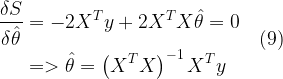
Thus, the least squared estimate of θ is given by
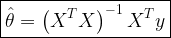
where the operator T denotes Hermitian Transpose (conjugate transpose).
Summary of computations
- Step 1: Choice of variables. Choose the variable to be explained (y) and the explanatory variables { x1, x2 ,…, xk } where x1 is often considered a constant (optional) that always takes the value 1 – this is to incorporate a DC component in the model.
- Step 2: Collect data. Collect n observations of y and for a set of known values of { x1, x2 ,…, xk }. Example: { x1, x2 ,…, xk } is the pilot data in OFDM using which we would like to estimate the channel impulse response θ and y is the received vector of samples. Store the observed data y in an – n⨉1 vector and the data on the explanatory variables in the n⨉k matrix X.
- Step 3: Compute the estimates. Compute the least squares estimates by the formula
The superscript T indicates Hermitian Transpose (conjugate transpose) operation.
Key Points
- We do not need a probabilistic assumption but only a deterministic signal model.
- It has a broader range of applications.
- Least squares is unbiased.
- Estimating the disturbance variance (k variables to estimate and n observations are available).
- To keep the variance low, the number of observations must be greater than the number of variables to estimate.
- The observation matrix X should have maximum rank – this leads to independent rows and columns which always happens with real data. This will make sure (XTX) is invertible.
- Least Squares Estimator can be used in block processing mode with overlapping segments – similar to Welch’s method of PSD estimation.
- Useful in time-frequency analysis.
- Adaptive filters are utilized for non-stationary applications.

LSE applied to curve fitting
Matlab snippet for implementing Least Estimate to fit a curve is given below.
x = -5:.1:5; % set of x- values - known explanatory variables
y = 5.3 + 1.2* x; % Straight line without noise
e=randn(size(y));
y = y + e; % adding random noise to get observed variable -
%Linear model - Y=Xa+e where a - parameters to be estimated

X = [ ones(length(x),1) x']; %first column treated aas all ones since x_1=1
y = y'; %column vector for proper dimension during multiplication
a = inv(X'*X)*X'*y  % Least Squares Estimator - equivalent code Xy
h=plot ( x , y , 'o'); %original data
hold on;
plot( x , a(1)+ a(2)*x , 'r-' ); %Fitted line
legend('observed samples',['y=' num2str(a(1)) '+' num2str(a(2)) 'x'])
title('Least Squares Estimate for Curve Fitting');
xlabel('X values');
ylabel('Y values');
Simulation Results

Rate this article: 
 (6 votes, average: 4.67 out of 5)
Related topics:
| [1] | An Introduction to Estimation Theory |
| [2] | Bias of an Estimator |
| [3] | Minimum Variance Unbiased Estimators (MVUE) |
| [4] | Maximum Likelihood Estimation |
| [5] | Maximum Likelihood Decoding |
| [6] | Probability and Random Process |
| [7] | Likelihood Function and Maximum Likelihood Estimation (MLE) |
| [8] | Score, Fisher Information and Estimator Sensitivity |
| [9] | Introduction to Cramer Rao Lower Bound (CRLB) |
| [10] | Cramer Rao Lower Bound for Scalar Parameter Estimation |
| [11] | Applying Cramer Rao Lower Bound (CRLB) to find a Minimum Variance Unbiased Estimator (MVUE) |
| [12] | Efficient Estimators and CRLB |
| [13] | Cramer Rao Lower Bound for Phase Estimation |
| [14] | Normalized CRLB — an alternate form of CRLB and its relation to estimator sensitivity |
| [15] | Cramer Rao Lower Bound (CRLB) for Vector Parameter Estimation |
| [16] | The Mean Square Error – Why do we use it for estimation problems |
| [17] | How to estimate unknown parameters using Ordinary Least Squares (OLS) |
| [18] | Essential Preliminary Matrix Algebra for Signal Processing |
| [19] | Why Cholesky Decomposition ? A sample case: |
| [20] | Tests for Positive Definiteness of a Matrix |
| [21] | Solving a Triangular Matrix using Forward & Backward Substitution |
| [22] | Cholesky Factorization — Matlab and Python |
| [23] | LTI system models for random signals – AR, MA and ARMA models |
| [24] | Comparing AR and ARMA model — minimization of squared error |
| [25] | Yule Walker Estimation |
| [26] | AutoCorrelation (Correlogram) and persistence – Time series analysis |
| [27] | Linear Models — Least Squares Estimator (LSE) |
| [28] | Best Linear Unbiased Estimator (BLUE) |