Материал из MachineLearning.
Перейти к: навигация, поиск
Содержание
- 1 Введение
- 2 Распространение ошибок
- 2.1 Абсолютная ошибка
- 2.2 Относительная ошибка
- 3 Графы вычислительных процессов
- 3.1 Примеры
- 4 Памятка программисту
- 5 Список литературы
- 6 См. также
Введение
Одним из наиболее важных вопросов в численном анализе является вопрос о том, как ошибка, возникшая в определенном месте в ходе вычислений, распространяется дальше, то есть становится ли ее влияние больше или меньше по мере того, как производятся последующие операции. Крайним случаем является вычитание двух почти равных чисел: даже при очень маленьких ошибках обоих этих чисел относительная ошибка разности может оказаться очень большой. Такая относительная ошибка будет распространяться дальше при выполнении всех последующих арифметических операций.
Одним из источников вычислительных погрешностей (ошибок) является приближенное представление вещественных чисел в ЭВМ, обусловленное конечностью разрядной сетки. Хотя исходные данные представляются в ЭВМ с большой точностью накопление погрешностей округления в процессе счета может привести к значительной результирующей погрешности, а некоторые алгоритмы могут оказаться и вовсе непригодными для реального счета на ЭВМ. Подробнее о представлении вещественных чисел в ЭВМ можно узнать здесь.
Распространение ошибок
В качестве первого шага при рассмотрении такого вопроса, как распространение ошибок, необходимо найти выражения для абсолютной и относительной ошибок результата каждого из четырех арифметических действий как функции величин, участвющих в операции, и их ошибок.
Абсолютная ошибка
Сложение
Имеются два приближения  и к двум величинам и , а также соответствующие абсолютные ошибки и . Тогда в результате сложения имеем
- .
Ошибка суммы, которую мы обозначим через , будет равна
- .
Вычитание
Тем же путем получаем
- .
Умножение
При умножении мы имеем
- .
Поскольку ошибки обычно гораздо меньше самих величин, пренебрегаем произведением ошибок:
- .
Ошибка произведения будет равна
- .
Деление
Имеем
- .
Преобразовываем это выражение к виду
- .
Множитель, стоящий в скобках, при можно разложить в ряд
- .
Перемножая и пренебрегая всеми членами, которые содержат произведения ошибок или степени ошибок выше первой, имеем
- .
Следовательно,
- .
Необходимо четко понимать, что знак ошибки бывает известен только в очень редких случаях. Не факт, например, что ошибка увеличивается при сложении и уменьшается при вычитании потому, что в формуле для сложения стоит плюс, а для вычитания — минус. Если, например, ошибки двух чисел имеют противоположные знаки, то дело будет обстоять как раз наоборот, то есть ошибка уменьшится при сложении и увеличится при вычитании этих чисел.
Относительная ошибка
После того, как мы вывели формулы для распространения абсолютных ошибок при четырех арифметических действиях, довольно просто вывести соответствующие формулы для относительных ошибок. Для сложения и вычитания формулы были преобразованы с тем, чтобы в них входила в явном виде относительная ошибка каждого исходного числа.
Сложение
- .
Вычитание
- .
Умножение
- .
Деление
- .
Мы начинаем арифметическую операцию, имея в своем распоряжении два приближенных значения и с соответствующими ошибками и . Ошибки эти могут быть любого происхождения. Величины и могут быть экспериментальными результатами, содержащими ошибки; они могут быть результатами предварительного вычисления согласно какому-либо бесконечному процессу и поэтому могут содержать ошибки ограничения; они могут быть результатами предшествующих арифметических операций и могут содержать ошибки округления. Естественно, они могут также содержать в различных комбинациях и все три вида ошибок.
Вышеприведенные формулы дают выражение ошибки результата каждого из четырех арифметических действий как функции от ; ошибка округления в данном арифметическом действии при этом не учитывается. Если же в дальнейшем необходимо будет подсчитать, как распространяется в последующих арифметических операциях ошибка этого результата, то необходимо к вычисленной по одной из четырех формул ошибке результата прибавить отдельно ошибку округления.
Графы вычислительных процессов
Теперь рассмотрим удобный способ подсчета распространения ошибки в каком-либо арифметическом вычислении. С этой целью мы будем изображать последовательность операций в вычислении с помощью графа и будем писать около стрелок графа коэффициенты, которые позволят нам сравнительно легко определить общую ошибку окончательного результата. Метод этот удобен еще и тем, что позволяет легко определить вклад любой ошибки, возникшей в процессе вычислений, в общую ошибку.
![]()
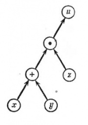
Рис.1. Граф вычислительного процесса
На рис.1 изображен граф вычислительного процесса . Граф следует читать снизу вверх, следуя стрелкам. Сначала выполняются операции, расположенные на каком-либо горизонтальном уровне, после этого — операции, расположенные на более высоком уровне, и т. д. Из рис.1, например, ясно, что x и y сначала складываются, а потом умножаются на z. Граф, изображенный на рис.1, является только изображением самого вычислительного процесса. Для подсчета общей ошибки результата необходимо дополнить этот граф коэффициентами, которые пишутся около стрелок согласно следующим правилам.
Сложение
Пусть две стрелки, которые входят в кружок сложения, выходят из двух кружков с величинами и . Эти величины могут быть как исходными, так и результатами предыдущих вычислений. Тогда стрелка, ведущая от к знаку + в кружке, получает коэффициент , стрелка же, ведущая от к знаку + в кружке, получает коэффициент .
Вычитание
Если выполняется операция , то соответствующие стрелки получают коэффициенты и .
Умножение
Обе стрелки, входящие в кружок умножения, получают коэффициент +1.
Деление
Если выполняется деление , то стрелка от к косой черте в кружке получает коэффициент +1, а стрелка от к косой черте в кружке получает коэффициент −1.
Смысл всех этих коэффициентов следующий: относительная ошибка результата любой операции (кружка) входит в результат следующей операции, умножаясь на коэффициенты у стрелки, соединяющей эти две операции.
Примеры
![]()
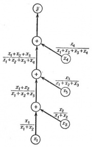
Рис.2. Граф вычислительного процесса для сложения , причем
Применим теперь методику графов к примерам и проиллюстрируем, что означает распространение ошибки в практических вычислениях.
Пример 1
Рассмотрим задачу сложения четырех положительных чисел:
- ,
где
- .
Граф этого процесса изображен на рис.2. Предположим, что все исходные величины заданы точно и не имеют ошибок, и пусть , и являются относительными ошибками округления после каждой следующей операции сложения. Последовательное применение правила для подсчета полной ошибки окончательного результата приводит к формуле
- .
Сокращая сумму в первом члене и умножая все выражение на , получаем
- .
Учитывая, что ошибка округления равна (в данном случае предполагается, что действительное число в ЭВМ представляется в виде десятичной дроби с t значищими цифрами), окончательно имеем
- .
Из этой формулы ясно, что максимально возможная ошибка (абсолютная или относительная), обусловленная округлением, становится меньше, если сначала складывать меньшие числа. Результат довольно удивительный, так как вся классическая математика основана на предположении, что при перемене мест слагаемых или их группировке сумма не изменяется. Разница заключается в том, что ЭВМ не может производить вычисления с бесконечно большой точностью, а именно такие вычисления рассматриваются в классической математике.
Пример 2
Вычитание двух почти равных чисел. Предположим, что необходимо вычислить . Тогда из формулы распространения ошибки при вычитании имеем
- .
Предположим, кроме того, что x и y являются соответствующим образом округленными положительными числами, так что
- и .
Если разность x-y мала, то относительная ошибка z может стать большой, даже если абсолютная ошибка мала. Так как в дальнейших вычислениях эта большая относительная ошибка будет распространяться, то она может поставить под сомнение точность окончательного результата вычислений.
Рассмотрим простой пример:
Тогда
Зная x и y, мы можем написать
Как видим, относительные ошибки x и y малы. Однако
Эта относительная ошибка очень велика, и, что важнее всего, она будет распространяться в ходе последующих вычислений.
Памятка программисту
Выводы, полученные выше, можно свести в краткий перечень рекомендаций для практической организации вычислений.
- Если необходимо произвести сложение-вычитание длинной последовательности чисел, работайте сначала с наименьшими числами.
- Если возможно, избегайте вычитания двух почти равных чисел. Формулы, содержащие такое вычитание, часто можно преобразовать так, чтобы избежать подобной операции.
- Выражение вида можно написать в виде , а выражение вида можно написать в виде . Если числа в разности почти равны друг другу, производите вычитание до умножения или деления. При этом задача не будет осложнена дополнительными ошибками округления.
- В любом случае сводите к минимуму число необходимых арифметических операций.
Список литературы
- Д.Мак-Кракен, У.Дорн. Численные методы и программирование на Фортране. Москва «Мир», 1977
- А. А. Самарский, А. В. Гулин. Численные методы. Москва «Наука», 1989.
См. также
- Практикум ММП ВМК, 4й курс, осень 2008
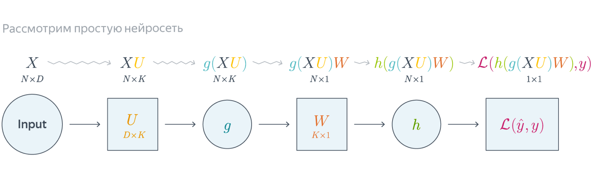
Нейронные сети обучаются с помощью тех или иных модификаций градиентного спуска, а чтобы применять его, нужно уметь эффективно вычислять градиенты функции потерь по всем обучающим параметрам. Казалось бы, для какого-нибудь запутанного вычислительного графа это может быть очень сложной задачей, но на помощь спешит метод обратного распространения ошибки.
Открытие метода обратного распространения ошибки стало одним из наиболее значимых событий в области искусственного интеллекта. В актуальном виде он был предложен в 1986 году Дэвидом Э. Румельхартом, Джеффри Э. Хинтоном и Рональдом Дж. Вильямсом и независимо и одновременно красноярскими математиками С. И. Барцевым и В. А. Охониным. С тех пор для нахождения градиентов параметров нейронной сети используется метод вычисления производной сложной функции, и оценка градиентов параметров сети стала хоть сложной инженерной задачей, но уже не искусством. Несмотря на простоту используемого математического аппарата, появление этого метода привело к значительному скачку в развитии искусственных нейронных сетей.
Суть метода можно записать одной формулой, тривиально следующей из формулы производной сложной функции: если $f(x) = g_m(g_{m-1}(ldots (g_1(x)) ldots))$, то $frac{partial f}{partial x} = frac{partial g_m}{partial g_{m-1}}frac{partial g_{m-1}}{partial g_{m-2}}ldots frac{partial g_2}{partial g_1}frac{partial g_1}{partial x}$. Уже сейчас мы видим, что градиенты можно вычислять последовательно, в ходе одного обратного прохода, начиная с $frac{partial g_m}{partial g_{m-1}}$ и умножая каждый раз на частные производные предыдущего слоя.
Backpropagation в одномерном случае
В одномерном случае всё выглядит особенно просто. Пусть $w_0$ — переменная, по которой мы хотим продифференцировать, причём сложная функция имеет вид
$$f(w_0) = g_m(g_{m-1}(ldots g_1(w_0)ldots)),$$
где все $g_i$ скалярные. Тогда
$$f'(w_0) = g_m'(g_{m-1}(ldots g_1(w_0)ldots))cdot g’_{m-1}(g_{m-2}(ldots g_1(w_0)ldots))cdotldots cdot g’_1(w_0)$$
Суть этой формулы такова. Если мы уже совершили forward pass, то есть уже знаем
$$g_1(w_0), g_2(g_1(w_0)),ldots,g_{m-1}(ldots g_1(w_0)ldots),$$
то мы действуем следующим образом:
-
берём производную $g_m$ в точке $g_{m-1}(ldots g_1(w_0)ldots)$;
-
умножаем на производную $g_{m-1}$ в точке $g_{m-2}(ldots g_1(w_0)ldots)$;
-
и так далее, пока не дойдём до производной $g_1$ в точке $w_0$.
Проиллюстрируем это на картинке, расписав по шагам дифференцирование по весам $w_i$ функции потерь логистической регрессии на одном объекте (то есть для батча размера 1):
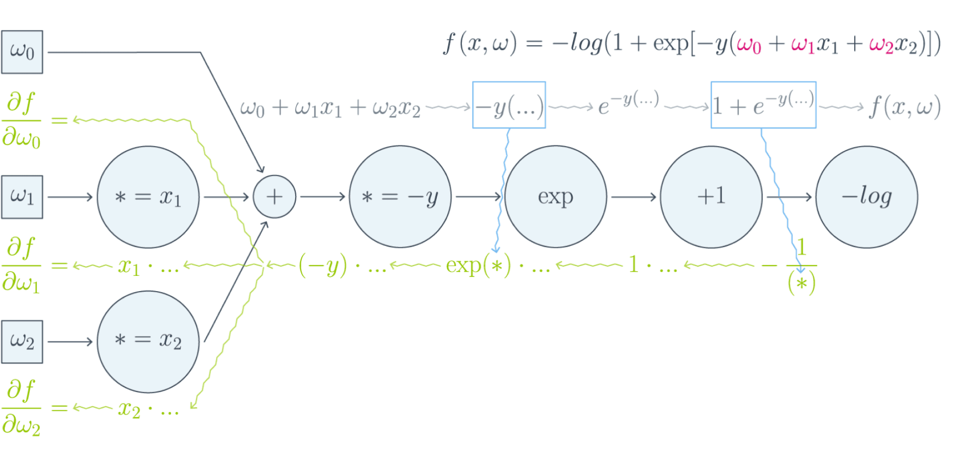
Собирая все множители вместе, получаем:
$$frac{partial f}{partial w_0} = (-y)cdot e^{-y(w_0 + w_1x_1 + w_2x_2)}cdotfrac{-1}{1 + e^{-y(w_0 + w_1x_1 + w_2x_2)}}$$
$$frac{partial f}{partial w_1} = x_1cdot(-y)cdot e^{-y(w_0 + w_1x_1 + w_2x_2)}cdotfrac{-1}{1 + e^{-y(w_0 + w_1x_1 + w_2x_2)}}$$
$$frac{partial f}{partial w_2} = x_2cdot(-y)cdot e^{-y(w_0 + w_1x_1 + w_2x_2)}cdotfrac{-1}{1 + e^{-y(w_0 + w_1x_1 + w_2x_2)}}$$
Таким образом, мы видим, что сперва совершается forward pass для вычисления всех промежуточных значений (и да, все промежуточные представления нужно будет хранить в памяти), а потом запускается backward pass, на котором в один проход вычисляются все градиенты.
Почему же нельзя просто пойти и начать везде вычислять производные?
В главе, посвящённой матричным дифференцированиям, мы поднимаем вопрос о том, что вычислять частные производные по отдельности — это зло, лучше пользоваться матричными вычислениями. Но есть и ещё одна причина: даже и с матричной производной в принципе не всегда хочется иметь дело. Рассмотрим простой пример. Допустим, что $X^r$ и $X^{r+1}$ — два последовательных промежуточных представления $Ntimes M$ и $Ntimes K$, связанных функцией $X^{r+1} = f^{r+1}(X^r)$. Предположим, что мы как-то посчитали производную $frac{partialmathcal{L}}{partial X^{r+1}_{ij}}$ функции потерь $mathcal{L}$, тогда
$$frac{partialmathcal{L}}{partial X^{r}_{st}} = sum_{i,j}frac{partial f^{r+1}_{ij}}{partial X^{r}_{st}}frac{partialmathcal{L}}{partial X^{r+1}_{ij}}$$
И мы видим, что, хотя оба градиента $frac{partialmathcal{L}}{partial X_{ij}^{r+1}}$ и $frac{partialmathcal{L}}{partial X_{st}^{r}}$ являются просто матрицами, в ходе вычислений возникает «четырёхмерный кубик» $frac{partial f_{ij}^{r+1}}{partial X_{st}^{r}}$, даже хранить который весьма болезненно: уж больно много памяти он требует ($N^2MK$ по сравнению с безобидными $NM + NK$, требуемыми для хранения градиентов). Поэтому хочется промежуточные производные $frac{partial f^{r+1}}{partial X^{r}}$ рассматривать не как вычисляемые объекты $frac{partial f_{ij}^{r+1}}{partial X_{st}^{r}}$, а как преобразования, которые превращают $frac{partialmathcal{L}}{partial X_{ij}^{r+1}}$ в $frac{partialmathcal{L}}{partial X_{st}^{r}}$. Целью следующих глав будет именно это: понять, как преобразуется градиент в ходе error backpropagation при переходе через тот или иной слой.
Вы спросите себя: надо ли мне сейчас пойти и прочитать главу учебника про матричное дифференцирование?
Встречный вопрос. Найдите производную функции по вектору $x$:
$$f(x) = x^TAx, Ain Mat_{n}{mathbb{R}}text{ — матрица размера }ntimes n$$
А как всё поменяется, если $A$ тоже зависит от $x$? Чему равен градиент функции, если $A$ является скаляром? Если вы готовы прямо сейчас взять ручку и бумагу и посчитать всё, то вам, вероятно, не надо читать про матричные дифференцирования. Но мы советуем всё-таки заглянуть в эту главу, если обозначения, которые мы будем дальше использовать, покажутся вам непонятными: единой нотации для матричных дифференцирований человечество пока, увы, не изобрело, и переводить с одной на другую не всегда легко.
Мы же сразу перейдём к интересующей нас вещи: к вычислению градиентов сложных функций.
Градиент сложной функции
Напомним, что формула производной сложной функции выглядит следующим образом:
$$left[D_{x_0} (color{#5002A7}{u} circ color{#4CB9C0}{v}) right](h) = color{#5002A7}{left[D_{v(x_0)} u right]} left( color{#4CB9C0}{left[D_{x_0} vright]} (h)right)$$
Теперь разберёмся с градиентами. Пусть $f(x) = g(h(x))$ – скалярная функция. Тогда
$$left[D_{x_0} f right] (x-x_0) = langlenabla_{x_0} f, x-x_0rangle.$$
С другой стороны,
$$left[D_{h(x_0)} g right] left(left[D_{x_0}h right] (x-x_0)right) = langlenabla_{h_{x_0}} g, left[D_{x_0} hright] (x-x_0)rangle = langleleft[D_{x_0} hright]^* nabla_{h(x_0)} g, x-x_0rangle.$$
То есть $color{#FFC100}{nabla_{x_0} f} = color{#348FEA}{left[D_{x_0} h right]}^* color{#FFC100}{nabla_{h(x_0)}}g$ — применение сопряжённого к $D_{x_0} h$ линейного отображения к вектору $nabla_{h(x_0)} g$.
Эта формула — сердце механизма обратного распространения ошибки. Она говорит следующее: если мы каким-то образом получили градиент функции потерь по переменным из некоторого промежуточного представления $X^k$ нейронной сети и при этом знаем, как преобразуется градиент при проходе через слой $f^k$ между $X^{k-1}$ и $X^k$ (то есть как выглядит сопряжённое к дифференциалу слоя между ними отображение), то мы сразу же находим градиент и по переменным из $X^{k-1}$:
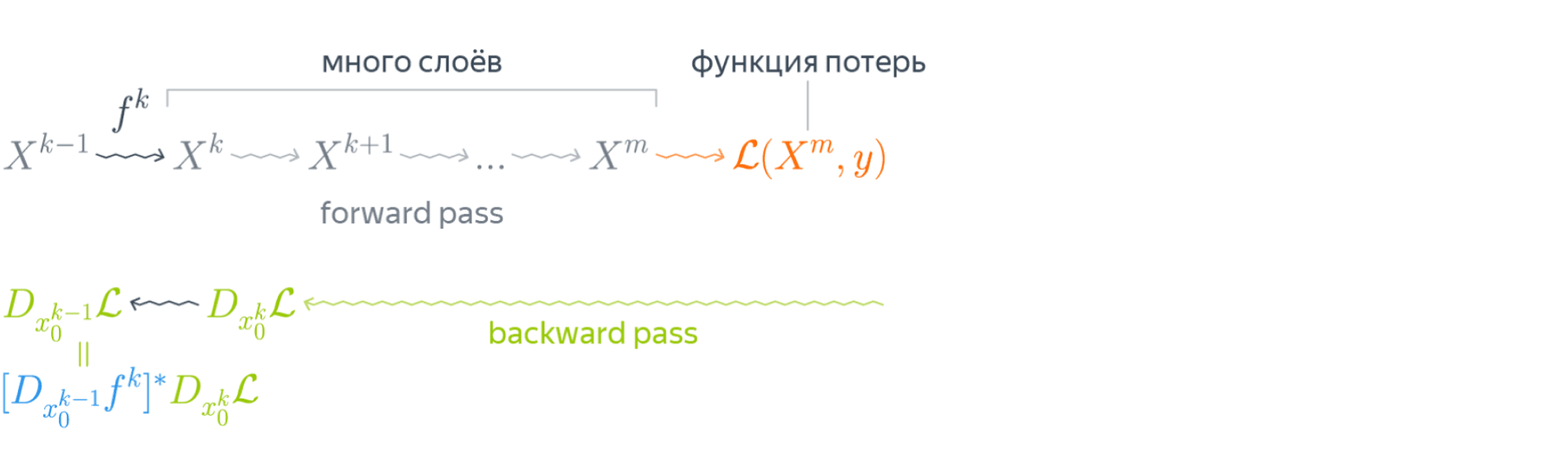
Таким образом слой за слоем мы посчитаем градиенты по всем $X^i$ вплоть до самых первых слоёв.
Далее мы разберёмся, как именно преобразуются градиенты при переходе через некоторые распространённые слои.
Градиенты для типичных слоёв
Рассмотрим несколько важных примеров.
Примеры
-
$f(x) = u(v(x))$, где $x$ — вектор, а $v(x)$ – поэлементное применение $v$:
$$vbegin{pmatrix}
x_1
vdots
x_N
end{pmatrix}
= begin{pmatrix}
v(x_1)
vdots
v(x_N)
end{pmatrix}$$Тогда, как мы знаем,
$$left[D_{x_0} fright] (h) = langlenabla_{x_0} f, hrangle = left[nabla_{x_0} fright]^T h.$$
Следовательно,
$$begin{multline*}
left[D_{v(x_0)} uright] left( left[ D_{x_0} vright] (h)right) = left[nabla_{v(x_0)} uright]^T left(v'(x_0) odot hright) =\[0.1cm]
= sumlimits_i left[nabla_{v(x_0)} uright]_i v'(x_{0i})h_i
= langleleft[nabla_{v(x_0)} uright] odot v'(x_0), hrangle.
end{multline*},$$где $odot$ означает поэлементное перемножение. Окончательно получаем
$$color{#348FEA}{nabla_{x_0} f = left[nabla_{v(x_0)}uright] odot v'(x_0) = v'(x_0) odot left[nabla_{v(x_0)} uright]}$$
Отметим, что если $x$ и $h(x)$ — это просто векторы, то мы могли бы вычислять всё и по формуле $frac{partial f}{partial x_i} = sum_jbig(frac{partial z_j}{partial x_i}big)cdotbig(frac{partial h}{partial z_j}big)$. В этом случае матрица $big(frac{partial z_j}{partial x_i}big)$ была бы диагональной (так как $z_j$ зависит только от $x_j$: ведь $h$ берётся поэлементно), и матричное умножение приводило бы к тому же результату. Однако если $x$ и $h(x)$ — матрицы, то $big(frac{partial z_j}{partial x_i}big)$ представлялась бы уже «четырёхмерным кубиком», и работать с ним было бы ужасно неудобно.
-
$f(X) = g(XW)$, где $X$ и $W$ — матрицы. Как мы знаем,
$$left[D_{X_0} f right] (X-X_0) = text{tr}, left(left[nabla_{X_0} fright]^T (X-X_0)right).$$
Тогда
$$begin{multline*}
left[ D_{X_0W} g right] left(left[D_{X_0} left( ast Wright)right] (H)right) =
left[ D_{X_0W} g right] left(HWright)=\
= text{tr}, left( left[nabla_{X_0W} g right]^T cdot (H) W right) =\
=
text{tr} , left(W left[nabla_{X_0W} (g) right]^T cdot (H)right) = text{tr} , left( left[left[nabla_{X_0W} gright] W^Tright]^T (H)right)
end{multline*}$$Здесь через $ast W$ мы обозначили отображение $Y hookrightarrow YW$, а в предпоследнем переходе использовалось следующее свойство следа:
$$
text{tr} , (A B C) = text{tr} , (C A B),
$$где $A, B, C$ — произвольные матрицы подходящих размеров (то есть допускающие перемножение в обоих приведённых порядках). Следовательно, получаем
$$color{#348FEA}{nabla_{X_0} f = left[nabla_{X_0W} (g) right] cdot W^T}$$
-
$f(W) = g(XW)$, где $W$ и $X$ — матрицы. Для приращения $H = W — W_0$ имеем
$$
left[D_{W_0} f right] (H) = text{tr} , left( left[nabla_{W_0} f right]^T (H)right)
$$Тогда
$$ begin{multline*}
left[D_{XW_0} g right] left( left[D_{W_0} left(X astright) right] (H)right) = left[D_{XW_0} g right] left( XH right) =
= text{tr} , left( left[nabla_{XW_0} g right]^T cdot X (H)right) =
text{tr}, left(left[X^T left[nabla_{XW_0} g right] right]^T (H)right)
end{multline*} $$Здесь через $X ast$ обозначено отображение $Y hookrightarrow XY$. Значит,
$$color{#348FEA}{nabla_{X_0} f = X^T cdot left[nabla_{XW_0} (g)right]}$$
-
$f(X) = g(softmax(X))$, где $X$ — матрица $Ntimes K$, а $softmax$ — функция, которая вычисляется построчно, причём для каждой строки $x$
$$softmax(x) = left(frac{e^{x_1}}{sum_te^{x_t}},ldots,frac{e^{x_K}}{sum_te^{x_t}}right)$$
В этом примере нам будет удобно воспользоваться формализмом с частными производными. Сначала вычислим $frac{partial s_l}{partial x_j}$ для одной строки $x$, где через $s_l$ мы для краткости обозначим $softmax(x)_l = frac{e^{x_l}} {sum_te^{x_t}}$. Нетрудно проверить, что
$$frac{partial s_l}{partial x_j} = begin{cases}
s_j(1 — s_j), & j = l,
-s_ls_j, & jne l
end{cases}$$Так как softmax вычисляется независимо от каждой строчки, то
$$frac{partial s_{rl}}{partial x_{ij}} = begin{cases}
s_{ij}(1 — s_{ij}), & r=i, j = l,
-s_{il}s_{ij}, & r = i, jne l,
0, & rne i
end{cases},$$где через $s_{rl}$ мы обозначили для краткости $softmax(X)_{rl}$.
Теперь пусть $nabla_{rl} = nabla g = frac{partialmathcal{L}}{partial s_{rl}}$ (пришедший со следующего слоя, уже известный градиент). Тогда
$$frac{partialmathcal{L}}{partial x_{ij}} = sum_{r,l}frac{partial s_{rl}}{partial x_{ij}} nabla_{rl}$$
Так как $frac{partial s_{rl}}{partial x_{ij}} = 0$ при $rne i$, мы можем убрать суммирование по $r$:
$$ldots = sum_{l}frac{partial s_{il}}{partial x_{ij}} nabla_{il} = -s_{i1}s_{ij}nabla_{i1} — ldots + s_{ij}(1 — s_{ij})nabla_{ij}-ldots — s_{iK}s_{ij}nabla_{iK} =$$
$$= -s_{ij}sum_t s_{it}nabla_{it} + s_{ij}nabla_{ij}$$
Таким образом, если мы хотим продифференцировать $f$ в какой-то конкретной точке $X_0$, то, смешивая математические обозначения с нотацией Python, мы можем записать:
$$begin{multline*}
color{#348FEA}{nabla_{X_0}f =}\
color{#348FEA}{= -softmax(X_0) odot text{sum}left(
softmax(X_0)odotnabla_{softmax(X_0)}g, text{ axis = 1}
right) +}\
color{#348FEA}{softmax(X_0)odot nabla_{softmax(X_0)}g}
end{multline*}
$$
Backpropagation в общем виде
Подытожим предыдущее обсуждение, описав алгоритм error backpropagation (алгоритм обратного распространения ошибки). Допустим, у нас есть текущие значения весов $W^i_0$ и мы хотим совершить шаг SGD по мини-батчу $X$. Мы должны сделать следующее:
- Совершить forward pass, вычислив и запомнив все промежуточные представления $X = X^0, X^1, ldots, X^m = widehat{y}$.
- Вычислить все градиенты с помощью backward pass.
- С помощью полученных градиентов совершить шаг SGD.
Проиллюстрируем алгоритм на примере двуслойной нейронной сети со скалярным output’ом. Для простоты опустим свободные члены в линейных слоях.
 Обучаемые параметры – матрицы $U$ и $W$. Как найти градиенты по ним в точке $U_0, W_0$?
$$nabla_{W_0}mathcal{L} = nabla_{W_0}{left({vphantom{frac12}mathcal{L}circ hcircleft[Wmapsto g(XU_0)Wright]}right)}=$$
$$=g(XU_0)^Tnabla_{g(XU_0)W_0}(mathcal{L}circ h) = underbrace{g(XU_0)^T}_{ktimes N}cdot
left[vphantom{frac12}underbrace{h’left(vphantom{int_0^1}g(XU_0)W_0right)}_{Ntimes 1}odot
underbrace{nabla_{hleft(vphantom{int_0^1}g(XU_0)W_0right)}mathcal{L}}_{Ntimes 1}right]$$
Итого матрица $ktimes 1$, как и $W_0$
$$nabla_{U_0}mathcal{L} = nabla_{U_0}left(vphantom{frac12}
mathcal{L}circ hcircleft[Ymapsto YW_0right]circ gcircleft[ Umapsto XUright]
right)=$$
$$=X^Tcdotnabla_{XU^0}left(vphantom{frac12}mathcal{L}circ hcirc [Ymapsto YW_0]circ gright) =$$
$$=X^Tcdotleft(vphantom{frac12}g'(XU_0)odot
nabla_{g(XU_0)}left[vphantom{in_0^1}mathcal{L}circ hcirc[Ymapsto YW_0right]
right)$$
$$=ldots = underset{Dtimes N}{X^T}cdotleft(vphantom{frac12}
underbrace{g'(XU_0)}_{Ntimes K}odot
underbrace{left[vphantom{int_0^1}left(
underbrace{h’left(vphantom{int_0^1}g(XU_0)W_0right)}_{Ntimes1}odotunderbrace{nabla_{h(vphantom{int_0^1}gleft(XU_0right)W_0)}mathcal{L}}_{Ntimes 1}
right)cdot underbrace{W^T}_{1times K}right]}_{Ntimes K}
right)$$
Итого $Dtimes K$, как и $U_0$
Схематически это можно представить следующим образом:
Backpropagation для двуслойной нейронной сети
Если вы не уследили за вычислениями в предыдущем примере, давайте более подробно разберём его чуть более конкретную версию (для $g = h = sigma$)Рассмотрим двуслойную нейронную сеть для классификации. Мы уже встречали ее ранее при рассмотрении линейно неразделимой выборки. Предсказания получаются следующим образом:
$$
widehat{y} = sigma(X^1 W^2) = sigmaBig(big(sigma(X^0 W^1 )big) W^2 Big).
$$
Пусть $W^1_0$ и $W^2_0$ — текущее приближение матриц весов. Мы хотим совершить шаг по градиенту функции потерь, и для этого мы должны вычислить её градиенты по $W^1$ и $W^2$ в точке $(W^1_0, W^2_0)$.
Прежде всего мы совершаем forward pass, в ходе которого мы должны запомнить все промежуточные представления: $X^1 = X^0 W^1_0$, $X^2 = sigma(X^0 W^1_0)$, $X^3 = sigma(X^0 W^1_0) W^2_0$, $X^4 = sigma(sigma(X^0 W^1_0) W^2_0) = widehat{y}$. Они понадобятся нам дальше.
Для полученных предсказаний вычисляется значение функции потерь:
$$
l = mathcal{L}(y, widehat{y}) = y log(widehat{y}) + (1-y) log(1-widehat{y}).
$$
Дальше мы шаг за шагом будем находить производные по переменным из всё более глубоких слоёв.
-
Градиент $mathcal{L}$ по предсказаниям имеет вид
$$
nabla_{widehat{y}}l = frac{y}{widehat{y}} — frac{1 — y}{1 — widehat{y}} = frac{y — widehat{y}}{widehat{y} (1 — widehat{y})},
$$где, напомним, $ widehat{y} = sigma(X^3) = sigmaBig(big(sigma(X^0 W^1_0 )big) W^2_0 Big)$ (обратите внимание на то, что $W^1_0$ и $W^2_0$ тут именно те, из которых мы делаем градиентный шаг).
-
Следующий слой — поэлементное взятие $sigma$. Как мы помним, при переходе через него градиент поэлементно умножается на производную $sigma$, в которую подставлено предыдущее промежуточное представление:
$$
nabla_{X^3}l = sigma'(X^3)odotnabla_{widehat{y}}l = sigma(X^3)left( 1 — sigma(X^3) right) odot frac{y — widehat{y}}{widehat{y} (1 — widehat{y})} =
$$$$
= sigma(X^3)left( 1 — sigma(X^3) right) odot frac{y — sigma(X^3)}{sigma(X^3) (1 — sigma(X^3))} =
y — sigma(X^3)
$$ -
Следующий слой — умножение на $W^2_0$. В этот момент мы найдём градиент как по $W^2$, так и по $X^2$. При переходе через умножение на матрицу градиент, как мы помним, умножается с той же стороны на транспонированную матрицу, а значит:
$$
color{blue}{nabla_{W^2_0}l} = (X^2)^Tcdot nabla_{X^3}l = (X^2)^Tcdot(y — sigma(X^3)) =
$$$$
= color{blue}{left( sigma(X^0W^1_0) right)^T cdot (y — sigma(sigma(X^0W^1_0)W^2_0))}
$$Аналогичным образом
$$
nabla_{X^2}l = nabla_{X^3}lcdot (W^2_0)^T = (y — sigma(X^3))cdot (W^2_0)^T =
$$$$
= (y — sigma(X^2W_0^2))cdot (W^2_0)^T
$$ -
Следующий слой — снова взятие $sigma$.
$$
nabla_{X^1}l = sigma'(X^1)odotnabla_{X^2}l = sigma(X^1)left( 1 — sigma(X^1) right) odot left( (y — sigma(X^2W_0^2))cdot (W^2_0)^T right) =
$$$$
= sigma(X^1)left( 1 — sigma(X^1) right) odotleft( (y — sigma(sigma(X^1)W_0^2))cdot (W^2_0)^T right)
$$ -
Наконец, последний слой — это умножение $X^0$ на $W^1_0$. Тут мы дифференцируем только по $W^1$:
$$
color{blue}{nabla_{W^1_0}l} = (X^0)^Tcdot nabla_{X^1}l = (X^0)^Tcdot big( sigma(X^1) left( 1 — sigma(X^1) right) odot (y — sigma(sigma(X^1)W_0^2))cdot (W^2_0)^Tbig) =
$$$$
= color{blue}{(X^0)^Tcdotbig(sigma(X^0W^1_0)left( 1 — sigma(X^0W^1_0) right) odot (y — sigma(sigma(X^0W^1_0)W_0^2))cdot (W^2_0)^Tbig) }
$$
Итоговые формулы для градиентов получились страшноватыми, но они были получены друг из друга итеративно с помощью очень простых операций: матричного и поэлементного умножения, в которые порой подставлялись значения заранее вычисленных промежуточных представлений.
Автоматизация и autograd
Итак, чтобы нейросеть обучалась, достаточно для любого слоя $f^k: X^{k-1}mapsto X^k$ с параметрами $W^k$ уметь:
- превращать $nabla_{X^k_0}mathcal{L}$ в $nabla_{X^{k-1}_0}mathcal{L}$ (градиент по выходу в градиент по входу);
- считать градиент по его параметрам $nabla_{W^k_0}mathcal{L}$.
При этом слою совершенно не надо знать, что происходит вокруг. То есть слой действительно может быть запрограммирован как отдельная сущность, умеющая внутри себя делать forward pass и backward pass, после чего слои механически, как кубики в конструкторе, собираются в большую сеть, которая сможет работать как одно целое.
Более того, во многих случаях авторы библиотек для глубинного обучения уже о вас позаботились и создали средства для автоматического дифференцирования выражений (autograd). Поэтому, программируя нейросеть, вы почти всегда можете думать только о forward-проходе, прямом преобразовании данных, предоставив библиотеке дифференцировать всё самостоятельно. Это делает код нейросетей весьма понятным и выразительным (да, в реальности он тоже бывает большим и страшным, но сравните на досуге код какой-нибудь разухабистой нейросети и код градиентного бустинга на решающих деревьях и почувствуйте разницу).
Но это лишь начало
Метод обратного распространения ошибки позволяет удобно посчитать градиенты, но дальше с ними что-то надо делать, и старый добрый SGD едва ли справится с обучением современной сетки. Так что же делать? О некоторых приёмах мы расскажем в следующей главе.
From Wikipedia, the free encyclopedia
In statistics, propagation of uncertainty (or propagation of error) is the effect of variables’ uncertainties (or errors, more specifically random errors) on the uncertainty of a function based on them. When the variables are the values of experimental measurements they have uncertainties due to measurement limitations (e.g., instrument precision) which propagate due to the combination of variables in the function.
The uncertainty u can be expressed in a number of ways.
It may be defined by the absolute error Δx. Uncertainties can also be defined by the relative error (Δx)/x, which is usually written as a percentage.
Most commonly, the uncertainty on a quantity is quantified in terms of the standard deviation, σ, which is the positive square root of the variance. The value of a quantity and its error are then expressed as an interval x ± u.
However, the most general way of characterizing uncertainty is by specifying its probability distribution.
If the probability distribution of the variable is known or can be assumed, in theory it is possible to get any of its statistics. In particular, it is possible to derive confidence limits to describe the region within which the true value of the variable may be found. For example, the 68% confidence limits for a one-dimensional variable belonging to a normal distribution are approximately ± one standard deviation σ from the central value x, which means that the region x ± σ will cover the true value in roughly 68% of cases.
If the uncertainties are correlated then covariance must be taken into account. Correlation can arise from two different sources. First, the measurement errors may be correlated. Second, when the underlying values are correlated across a population, the uncertainties in the group averages will be correlated.[1]
In a general context where a nonlinear function modifies the uncertain parameters (correlated or not), the standard tools to propagate uncertainty, and infer resulting quantity probability distribution/statistics, are sampling techniques from the Monte Carlo method family.[2] For very expensive data or complex functions, the calculation of the error propagation may be very expensive so that a surrogate model[3] or a parallel computing strategy[4][5][6] may be necessary.
In some particular cases, the uncertainty propagation calculation can be done through simplistic algebraic procedures. Some of these scenarios are described below.
Linear combinations[edit]
Let  be a set of m functions, which are linear combinations of
  variables
  with combination coefficients
  :
:

or in matrix notation,

Also let the variance–covariance matrix of x = (x1, …, xn) be denoted by  and let the mean value be denoted by
  :
:
![{displaystyle {boldsymbol {Sigma }}^{x}=E[mathbf {(x-mu )} otimes mathbf {(x-mu )} ]={begin{pmatrix}sigma _{1}^{2}&sigma _{12}&sigma _{13}&cdots \sigma _{21}&sigma _{2}^{2}&sigma _{23}&cdots \sigma _{31}&sigma _{32}&sigma _{3}^{2}&cdots \vdots &vdots &vdots &ddots end{pmatrix}}={begin{pmatrix}{Sigma }_{11}^{x}&{Sigma }_{12}^{x}&{Sigma }_{13}^{x}&cdots \{Sigma }_{21}^{x}&{Sigma }_{22}^{x}&{Sigma }_{23}^{x}&cdots \{Sigma }_{31}^{x}&{Sigma }_{32}^{x}&{Sigma }_{33}^{x}&cdots \vdots &vdots &vdots &ddots end{pmatrix}}.}](https://wikimedia.org/api/rest_v1/media/math/render/svg/cfac4652b328d3d5efe1c7bb8c226db7992be18e)
 is the outer product.
Then, the variance–covariance matrix  of f is given by
![{displaystyle {boldsymbol {Sigma }}^{f}=E[(mathbf {f} -E[mathbf {f} ])otimes (mathbf {f} -E[mathbf {f} ])]=E[mathbf {A(x-mu )} otimes mathbf {A(x-mu )} ]=mathbf {A} E[mathbf {(x-mu )} otimes mathbf {(x-mu )} ]mathbf {A} ^{mathrm {T} }=mathbf {A} {boldsymbol {Sigma }}^{x}mathbf {A} ^{mathrm {T} }}](https://wikimedia.org/api/rest_v1/media/math/render/svg/497583b88ad32fd41213cfd12e5293043f922408)
In component notation, the equation

reads

This is the most general expression for the propagation of error from one set of variables onto another. When the errors on x are uncorrelated, the general expression simplifies to

where  is the variance of k-th element of the x vector.
Note that even though the errors on x may be uncorrelated, the errors on f are in general correlated; in other words, even if is a diagonal matrix, is in general a full matrix.
The general expressions for a scalar-valued function f are a little simpler (here a is a row vector):


Each covariance term  can be expressed in terms of the correlation coefficient
  by
by  , so that an alternative expression for the variance of f is

In the case that the variables in x are uncorrelated, this simplifies further to

In the simple case of identical coefficients and variances, we find

For the arithmetic mean,  , the result is the standard error of the mean:

Non-linear combinations[edit]
When f is a set of non-linear combination of the variables x, an interval propagation could be performed in order to compute intervals which contain all consistent values for the variables. In a probabilistic approach, the function f must usually be linearised by approximation to a first-order Taylor series expansion, though in some cases, exact formulae can be derived that do not depend on the expansion as is the case for the exact variance of products.[7] The Taylor expansion would be:

where  denotes the partial derivative of fk with respect to the i-th variable, evaluated at the mean value of all components of vector x. Or in matrix notation,

where J is the Jacobian matrix. Since f0 is a constant it does not contribute to the error on f. Therefore, the propagation of error follows the linear case, above, but replacing the linear coefficients, Aki and Akj by the partial derivatives,  and
and  . In matrix notation,[8]

That is, the Jacobian of the function is used to transform the rows and columns of the variance-covariance matrix of the argument.
Note this is equivalent to the matrix expression for the linear case with  .
.
Simplification[edit]
Neglecting correlations or assuming independent variables yields a common formula among engineers and experimental scientists to calculate error propagation, the variance formula:[9]

where  represents the standard deviation of the function
  ,
,  represents the standard deviation of
  ,
,  represents the standard deviation of
  , and so forth.
It is important to note that this formula is based on the linear characteristics of the gradient of and therefore it is a good estimation for the standard deviation of as long as  are small enough. Specifically, the linear approximation of has to be close to inside a neighbourhood of radius .[10]
Example[edit]
Any non-linear differentiable function,  , of two variables,
  and
and  , can be expanded as

now, taking variance on both sides, and using the formula[11] for variance of a linear combination of variables:

hence:

where  is the standard deviation of the function ,
  is the standard deviation of ,
  is the standard deviation of and
  is the covariance between and .
In the particular case that  ,
,  . Then

or

where  is the correlation between and .
When the variables and are uncorrelated,  . Then

Caveats and warnings[edit]
Error estimates for non-linear functions are biased on account of using a truncated series expansion. The extent of this bias depends on the nature of the function. For example, the bias on the error calculated for log(1+x) increases as x increases, since the expansion to x is a good approximation only when x is near zero.
For highly non-linear functions, there exist five categories of probabilistic approaches for uncertainty propagation;[12] see Uncertainty quantification for details.
Reciprocal and shifted reciprocal[edit]
In the special case of the inverse or reciprocal  , where
  follows a standard normal distribution, the resulting distribution is a reciprocal standard normal distribution, and there is no definable variance.[13]
However, in the slightly more general case of a shifted reciprocal function  for
for  following a general normal distribution, then mean and variance statistics do exist in a principal value sense, if the difference between the pole
  and the mean
  is real-valued.[14]
Ratios[edit]
Ratios are also problematic; normal approximations exist under certain conditions.
Example formulae[edit]
This table shows the variances and standard deviations of simple functions of the real variables  , with standard deviations
  covariance
  , and correlation
  .
.
The real-valued coefficients and are assumed exactly known (deterministic), i.e.,  .
.
In the columns «Variance» and «Standard Deviation», A and B should be understood as expectation values (i.e. values around which we’re estimating the uncertainty), and should be understood as the value of the function calculated at the expectation value of .
-
Function Variance Standard Deviation
[15][16]
[17]
[18]
[18]
[19]


![{displaystyle sigma _{f}^{2}approx f^{2}left[left({frac {sigma _{A}}{A}}right)^{2}+left({frac {sigma _{B}}{B}}right)^{2}+2{frac {sigma _{AB}}{AB}}right]}](https://wikimedia.org/api/rest_v1/media/math/render/svg/9499339791864087918a8411cfc3d6d3d64adb4d)


![sigma _{f}^{2}approx f^{2}left[left({frac {sigma _{A}}{A}}right)^{2}+left({frac {sigma _{B}}{B}}right)^{2}-2{frac {sigma _{{AB}}}{AB}}right]](https://wikimedia.org/api/rest_v1/media/math/render/svg/1443509fb7b51ea477c6c24a17910bde4e81863a)


![{displaystyle sigma _{f}^{2}approx left[abcos(bA)sigma _{A}right]^{2}}](https://wikimedia.org/api/rest_v1/media/math/render/svg/02967f1c0ff2eb7edac9b2fad3bb020fb7fad0cf)


![{displaystyle sigma _{f}^{2}approx left[absin(bA)sigma _{A}right]^{2}}](https://wikimedia.org/api/rest_v1/media/math/render/svg/4f4d187dd08f03fd8b03cf3606cc9f166e5656aa)


![{displaystyle sigma _{f}^{2}approx left[absec ^{2}(bA)sigma _{A}right]^{2}}](https://wikimedia.org/api/rest_v1/media/math/render/svg/4308e87b0ada5699f04d64d6088e12e18fc7511f)


![sigma _{f}^{2}approx f^{2}left[left({frac {B}{A}}sigma _{A}right)^{2}+left(ln(A)sigma _{B}right)^{2}+2{frac {Bln(A)}{A}}sigma _{{AB}}right]](https://wikimedia.org/api/rest_v1/media/math/render/svg/977fba6a8423710573203b5286497b3ceffeb60e)


For uncorrelated variables ( ,
,  ) expressions for more complicated functions can be derived by combining simpler functions. For example, repeated multiplication, assuming no correlation, gives

For the case  we also have Goodman’s expression[7] for the exact variance: for the uncorrelated case it is

and therefore we have:

Effect of correlation on differences[edit]
If A and B are uncorrelated, their difference A-B will have more variance than either of them. An increasing positive correlation ( ) will decrease the variance of the difference, converging to zero variance for perfectly correlated variables with the same variance. On the other hand, a negative correlation (
 ) will further increase the variance of the difference, compared to the uncorrelated case.
For example, the self-subtraction f=A-A has zero variance  only if the variate is perfectly autocorrelated (
 ). If A is uncorrelated,
  , then the output variance is twice the input variance,
  . And if A is perfectly anticorrelated,
  , then the input variance is quadrupled in the output,
  (notice
  for f = aA — aA in the table above).
Example calculations[edit]
Inverse tangent function[edit]
We can calculate the uncertainty propagation for the inverse tangent function as an example of using partial derivatives to propagate error.
Define

where  is the absolute uncertainty on our measurement of x. The derivative of f(x) with respect to x is

Therefore, our propagated uncertainty is

where  is the absolute propagated uncertainty.
Resistance measurement[edit]
A practical application is an experiment in which one measures current, I, and voltage, V, on a resistor in order to determine the resistance, R, using Ohm’s law, R = V / I.
Given the measured variables with uncertainties, I ± σI and V ± σV, and neglecting their possible correlation, the uncertainty in the computed quantity, σR, is:

See also[edit]
- Accuracy and precision
- Automatic differentiation
- Bienaymé’s identity
- Delta method
- Dilution of precision (navigation)
- Errors and residuals in statistics
- Experimental uncertainty analysis
- Interval finite element
- Measurement uncertainty
- Numerical stability
- Probability bounds analysis
- Significance arithmetic
- Uncertainty quantification
- Random-fuzzy variable
- Variance#Propagation
References[edit]
- ^ Kirchner, James. «Data Analysis Toolkit #5: Uncertainty Analysis and Error Propagation» (PDF). Berkeley Seismology Laboratory. University of California. Retrieved 22 April 2016.
- ^ Kroese, D. P.; Taimre, T.; Botev, Z. I. (2011). Handbook of Monte Carlo Methods. John Wiley & Sons.
- ^ Ranftl, Sascha; von der Linden, Wolfgang (2021-11-13). «Bayesian Surrogate Analysis and Uncertainty Propagation». Physical Sciences Forum. 3 (1): 6. doi:10.3390/psf2021003006. ISSN 2673-9984.
- ^ Atanassova, E.; Gurov, T.; Karaivanova, A.; Ivanovska, S.; Durchova, M.; Dimitrov, D. (2016). «On the parallelization approaches for Intel MIC architecture». AIP Conference Proceedings. 1773 (1): 070001. Bibcode:2016AIPC.1773g0001A. doi:10.1063/1.4964983.
- ^ Cunha Jr, A.; Nasser, R.; Sampaio, R.; Lopes, H.; Breitman, K. (2014). «Uncertainty quantification through the Monte Carlo method in a cloud computing setting». Computer Physics Communications. 185 (5): 1355–1363. arXiv:2105.09512. Bibcode:2014CoPhC.185.1355C. doi:10.1016/j.cpc.2014.01.006. S2CID 32376269.
- ^ Lin, Y.; Wang, F.; Liu, B. (2018). «Random number generators for large-scale parallel Monte Carlo simulations on FPGA». Journal of Computational Physics. 360: 93–103. Bibcode:2018JCoPh.360…93L. doi:10.1016/j.jcp.2018.01.029.
- ^ a b Goodman, Leo (1960). «On the Exact Variance of Products». Journal of the American Statistical Association. 55 (292): 708–713. doi:10.2307/2281592. JSTOR 2281592.
- ^ Ochoa1,Benjamin; Belongie, Serge «Covariance Propagation for Guided Matching» Archived 2011-07-20 at the Wayback Machine
- ^ Ku, H. H. (October 1966). «Notes on the use of propagation of error formulas». Journal of Research of the National Bureau of Standards. 70C (4): 262. doi:10.6028/jres.070c.025. ISSN 0022-4316. Retrieved 3 October 2012.
- ^ Clifford, A. A. (1973). Multivariate error analysis: a handbook of error propagation and calculation in many-parameter systems. John Wiley & Sons. ISBN 978-0470160558.[page needed]
- ^ Soch, Joram (2020-07-07). «Variance of the linear combination of two random variables». The Book of Statistical Proofs. Retrieved 2022-01-29.
- ^ Lee, S. H.; Chen, W. (2009). «A comparative study of uncertainty propagation methods for black-box-type problems». Structural and Multidisciplinary Optimization. 37 (3): 239–253. doi:10.1007/s00158-008-0234-7. S2CID 119988015.
- ^ Johnson, Norman L.; Kotz, Samuel; Balakrishnan, Narayanaswamy (1994). Continuous Univariate Distributions, Volume 1. Wiley. p. 171. ISBN 0-471-58495-9.
- ^ Lecomte, Christophe (May 2013). «Exact statistics of systems with uncertainties: an analytical theory of rank-one stochastic dynamic systems». Journal of Sound and Vibration. 332 (11): 2750–2776. doi:10.1016/j.jsv.2012.12.009.
- ^ «A Summary of Error Propagation» (PDF). p. 2. Archived from the original (PDF) on 2016-12-13. Retrieved 2016-04-04.
- ^ «Propagation of Uncertainty through Mathematical Operations» (PDF). p. 5. Retrieved 2016-04-04.
- ^ «Strategies for Variance Estimation» (PDF). p. 37. Retrieved 2013-01-18.
- ^ a b Harris, Daniel C. (2003), Quantitative chemical analysis (6th ed.), Macmillan, p. 56, ISBN 978-0-7167-4464-1
- ^ «Error Propagation tutorial» (PDF). Foothill College. October 9, 2009. Retrieved 2012-03-01.
Further reading[edit]
- Bevington, Philip R.; Robinson, D. Keith (2002), Data Reduction and Error Analysis for the Physical Sciences (3rd ed.), McGraw-Hill, ISBN 978-0-07-119926-1
- Fornasini, Paolo (2008), The uncertainty in physical measurements: an introduction to data analysis in the physics laboratory, Springer, p. 161, ISBN 978-0-387-78649-0
- Meyer, Stuart L. (1975), Data Analysis for Scientists and Engineers, Wiley, ISBN 978-0-471-59995-1
- Peralta, M. (2012), Propagation Of Errors: How To Mathematically Predict Measurement Errors, CreateSpace
- Rouaud, M. (2013), Probability, Statistics and Estimation: Propagation of Uncertainties in Experimental Measurement (PDF) (short ed.)
- Taylor, J. R. (1997), An Introduction to Error Analysis: The Study of Uncertainties in Physical Measurements (2nd ed.), University Science Books
- Wang, C M; Iyer, Hari K (2005-09-07). «On higher-order corrections for propagating uncertainties». Metrologia. 42 (5): 406–410. doi:10.1088/0026-1394/42/5/011. ISSN 0026-1394.
External links[edit]
- A detailed discussion of measurements and the propagation of uncertainty explaining the benefits of using error propagation formulas and Monte Carlo simulations instead of simple significance arithmetic
- GUM, Guide to the Expression of Uncertainty in Measurement
- EPFL An Introduction to Error Propagation, Derivation, Meaning and Examples of Cy = Fx Cx Fx’
- uncertainties package, a program/library for transparently performing calculations with uncertainties (and error correlations).
- soerp package, a Python program/library for transparently performing *second-order* calculations with uncertainties (and error correlations).
- Joint Committee for Guides in Metrology (2011). JCGM 102: Evaluation of Measurement Data — Supplement 2 to the «Guide to the Expression of Uncertainty in Measurement» — Extension to Any Number of Output Quantities (PDF) (Technical report). JCGM. Retrieved 13 February 2013.
- Uncertainty Calculator Propagate uncertainty for any expression
From Wikipedia, the free encyclopedia
In statistics, propagation of uncertainty (or propagation of error) is the effect of variables’ uncertainties (or errors, more specifically random errors) on the uncertainty of a function based on them. When the variables are the values of experimental measurements they have uncertainties due to measurement limitations (e.g., instrument precision) which propagate due to the combination of variables in the function.
The uncertainty u can be expressed in a number of ways.
It may be defined by the absolute error Δx. Uncertainties can also be defined by the relative error (Δx)/x, which is usually written as a percentage.
Most commonly, the uncertainty on a quantity is quantified in terms of the standard deviation, σ, which is the positive square root of the variance. The value of a quantity and its error are then expressed as an interval x ± u.
However, the most general way of characterizing uncertainty is by specifying its probability distribution.
If the probability distribution of the variable is known or can be assumed, in theory it is possible to get any of its statistics. In particular, it is possible to derive confidence limits to describe the region within which the true value of the variable may be found. For example, the 68% confidence limits for a one-dimensional variable belonging to a normal distribution are approximately ± one standard deviation σ from the central value x, which means that the region x ± σ will cover the true value in roughly 68% of cases.
If the uncertainties are correlated then covariance must be taken into account. Correlation can arise from two different sources. First, the measurement errors may be correlated. Second, when the underlying values are correlated across a population, the uncertainties in the group averages will be correlated.[1]
In a general context where a nonlinear function modifies the uncertain parameters (correlated or not), the standard tools to propagate uncertainty, and infer resulting quantity probability distribution/statistics, are sampling techniques from the Monte Carlo method family.[2] For very expensive data or complex functions, the calculation of the error propagation may be very expensive so that a surrogate model[3] or a parallel computing strategy[4][5][6] may be necessary.
In some particular cases, the uncertainty propagation calculation can be done through simplistic algebraic procedures. Some of these scenarios are described below.
Linear combinations[edit]
Let be a set of m functions, which are linear combinations of variables with combination coefficients :
or in matrix notation,
Also let the variance–covariance matrix of x = (x1, …, xn) be denoted by and let the mean value be denoted by :
is the outer product.
Then, the variance–covariance matrix of f is given by
In component notation, the equation
reads
This is the most general expression for the propagation of error from one set of variables onto another. When the errors on x are uncorrelated, the general expression simplifies to
where is the variance of k-th element of the x vector.
Note that even though the errors on x may be uncorrelated, the errors on f are in general correlated; in other words, even if is a diagonal matrix, is in general a full matrix.
The general expressions for a scalar-valued function f are a little simpler (here a is a row vector):
Each covariance term can be expressed in terms of the correlation coefficient by , so that an alternative expression for the variance of f is
In the case that the variables in x are uncorrelated, this simplifies further to
In the simple case of identical coefficients and variances, we find
For the arithmetic mean, , the result is the standard error of the mean:
Non-linear combinations[edit]
When f is a set of non-linear combination of the variables x, an interval propagation could be performed in order to compute intervals which contain all consistent values for the variables. In a probabilistic approach, the function f must usually be linearised by approximation to a first-order Taylor series expansion, though in some cases, exact formulae can be derived that do not depend on the expansion as is the case for the exact variance of products.[7] The Taylor expansion would be:
where denotes the partial derivative of fk with respect to the i-th variable, evaluated at the mean value of all components of vector x. Or in matrix notation,
where J is the Jacobian matrix. Since f0 is a constant it does not contribute to the error on f. Therefore, the propagation of error follows the linear case, above, but replacing the linear coefficients, Aki and Akj by the partial derivatives, and . In matrix notation,[8]
That is, the Jacobian of the function is used to transform the rows and columns of the variance-covariance matrix of the argument.
Note this is equivalent to the matrix expression for the linear case with .
Simplification[edit]
Neglecting correlations or assuming independent variables yields a common formula among engineers and experimental scientists to calculate error propagation, the variance formula:[9]
where represents the standard deviation of the function , represents the standard deviation of , represents the standard deviation of , and so forth.
It is important to note that this formula is based on the linear characteristics of the gradient of and therefore it is a good estimation for the standard deviation of as long as are small enough. Specifically, the linear approximation of has to be close to inside a neighbourhood of radius .[10]
Example[edit]
Any non-linear differentiable function, , of two variables, and , can be expanded as
now, taking variance on both sides, and using the formula[11] for variance of a linear combination of variables:
hence:
where is the standard deviation of the function , is the standard deviation of , is the standard deviation of and is the covariance between and .
In the particular case that , . Then
or
where is the correlation between and .
When the variables and are uncorrelated, . Then
Caveats and warnings[edit]
Error estimates for non-linear functions are biased on account of using a truncated series expansion. The extent of this bias depends on the nature of the function. For example, the bias on the error calculated for log(1+x) increases as x increases, since the expansion to x is a good approximation only when x is near zero.
For highly non-linear functions, there exist five categories of probabilistic approaches for uncertainty propagation;[12] see Uncertainty quantification for details.
Reciprocal and shifted reciprocal[edit]
In the special case of the inverse or reciprocal , where follows a standard normal distribution, the resulting distribution is a reciprocal standard normal distribution, and there is no definable variance.[13]
However, in the slightly more general case of a shifted reciprocal function for following a general normal distribution, then mean and variance statistics do exist in a principal value sense, if the difference between the pole and the mean is real-valued.[14]
Ratios[edit]
Ratios are also problematic; normal approximations exist under certain conditions.
Example formulae[edit]
This table shows the variances and standard deviations of simple functions of the real variables , with standard deviations covariance , and correlation .
The real-valued coefficients and are assumed exactly known (deterministic), i.e., .
In the columns «Variance» and «Standard Deviation», A and B should be understood as expectation values (i.e. values around which we’re estimating the uncertainty), and should be understood as the value of the function calculated at the expectation value of .
-
Function Variance Standard Deviation
[15][16]
[17]
[18]
[18]
[19]
For uncorrelated variables (, ) expressions for more complicated functions can be derived by combining simpler functions. For example, repeated multiplication, assuming no correlation, gives
For the case we also have Goodman’s expression[7] for the exact variance: for the uncorrelated case it is
and therefore we have:
Effect of correlation on differences[edit]
If A and B are uncorrelated, their difference A-B will have more variance than either of them. An increasing positive correlation () will decrease the variance of the difference, converging to zero variance for perfectly correlated variables with the same variance. On the other hand, a negative correlation () will further increase the variance of the difference, compared to the uncorrelated case.
For example, the self-subtraction f=A-A has zero variance only if the variate is perfectly autocorrelated (). If A is uncorrelated, , then the output variance is twice the input variance, . And if A is perfectly anticorrelated, , then the input variance is quadrupled in the output, (notice for f = aA — aA in the table above).
Example calculations[edit]
Inverse tangent function[edit]
We can calculate the uncertainty propagation for the inverse tangent function as an example of using partial derivatives to propagate error.
Define
where is the absolute uncertainty on our measurement of x. The derivative of f(x) with respect to x is
Therefore, our propagated uncertainty is
where is the absolute propagated uncertainty.
Resistance measurement[edit]
A practical application is an experiment in which one measures current, I, and voltage, V, on a resistor in order to determine the resistance, R, using Ohm’s law, R = V / I.
Given the measured variables with uncertainties, I ± σI and V ± σV, and neglecting their possible correlation, the uncertainty in the computed quantity, σR, is:
See also[edit]
- Accuracy and precision
- Automatic differentiation
- Bienaymé’s identity
- Delta method
- Dilution of precision (navigation)
- Errors and residuals in statistics
- Experimental uncertainty analysis
- Interval finite element
- Measurement uncertainty
- Numerical stability
- Probability bounds analysis
- Significance arithmetic
- Uncertainty quantification
- Random-fuzzy variable
- Variance#Propagation
References[edit]
- ^ Kirchner, James. «Data Analysis Toolkit #5: Uncertainty Analysis and Error Propagation» (PDF). Berkeley Seismology Laboratory. University of California. Retrieved 22 April 2016.
- ^ Kroese, D. P.; Taimre, T.; Botev, Z. I. (2011). Handbook of Monte Carlo Methods. John Wiley & Sons.
- ^ Ranftl, Sascha; von der Linden, Wolfgang (2021-11-13). «Bayesian Surrogate Analysis and Uncertainty Propagation». Physical Sciences Forum. 3 (1): 6. doi:10.3390/psf2021003006. ISSN 2673-9984.
- ^ Atanassova, E.; Gurov, T.; Karaivanova, A.; Ivanovska, S.; Durchova, M.; Dimitrov, D. (2016). «On the parallelization approaches for Intel MIC architecture». AIP Conference Proceedings. 1773 (1): 070001. Bibcode:2016AIPC.1773g0001A. doi:10.1063/1.4964983.
- ^ Cunha Jr, A.; Nasser, R.; Sampaio, R.; Lopes, H.; Breitman, K. (2014). «Uncertainty quantification through the Monte Carlo method in a cloud computing setting». Computer Physics Communications. 185 (5): 1355–1363. arXiv:2105.09512. Bibcode:2014CoPhC.185.1355C. doi:10.1016/j.cpc.2014.01.006. S2CID 32376269.
- ^ Lin, Y.; Wang, F.; Liu, B. (2018). «Random number generators for large-scale parallel Monte Carlo simulations on FPGA». Journal of Computational Physics. 360: 93–103. Bibcode:2018JCoPh.360…93L. doi:10.1016/j.jcp.2018.01.029.
- ^ a b Goodman, Leo (1960). «On the Exact Variance of Products». Journal of the American Statistical Association. 55 (292): 708–713. doi:10.2307/2281592. JSTOR 2281592.
- ^ Ochoa1,Benjamin; Belongie, Serge «Covariance Propagation for Guided Matching» Archived 2011-07-20 at the Wayback Machine
- ^ Ku, H. H. (October 1966). «Notes on the use of propagation of error formulas». Journal of Research of the National Bureau of Standards. 70C (4): 262. doi:10.6028/jres.070c.025. ISSN 0022-4316. Retrieved 3 October 2012.
- ^ Clifford, A. A. (1973). Multivariate error analysis: a handbook of error propagation and calculation in many-parameter systems. John Wiley & Sons. ISBN 978-0470160558.[page needed]
- ^ Soch, Joram (2020-07-07). «Variance of the linear combination of two random variables». The Book of Statistical Proofs. Retrieved 2022-01-29.
- ^ Lee, S. H.; Chen, W. (2009). «A comparative study of uncertainty propagation methods for black-box-type problems». Structural and Multidisciplinary Optimization. 37 (3): 239–253. doi:10.1007/s00158-008-0234-7. S2CID 119988015.
- ^ Johnson, Norman L.; Kotz, Samuel; Balakrishnan, Narayanaswamy (1994). Continuous Univariate Distributions, Volume 1. Wiley. p. 171. ISBN 0-471-58495-9.
- ^ Lecomte, Christophe (May 2013). «Exact statistics of systems with uncertainties: an analytical theory of rank-one stochastic dynamic systems». Journal of Sound and Vibration. 332 (11): 2750–2776. doi:10.1016/j.jsv.2012.12.009.
- ^ «A Summary of Error Propagation» (PDF). p. 2. Archived from the original (PDF) on 2016-12-13. Retrieved 2016-04-04.
- ^ «Propagation of Uncertainty through Mathematical Operations» (PDF). p. 5. Retrieved 2016-04-04.
- ^ «Strategies for Variance Estimation» (PDF). p. 37. Retrieved 2013-01-18.
- ^ a b Harris, Daniel C. (2003), Quantitative chemical analysis (6th ed.), Macmillan, p. 56, ISBN 978-0-7167-4464-1
- ^ «Error Propagation tutorial» (PDF). Foothill College. October 9, 2009. Retrieved 2012-03-01.
Further reading[edit]
- Bevington, Philip R.; Robinson, D. Keith (2002), Data Reduction and Error Analysis for the Physical Sciences (3rd ed.), McGraw-Hill, ISBN 978-0-07-119926-1
- Fornasini, Paolo (2008), The uncertainty in physical measurements: an introduction to data analysis in the physics laboratory, Springer, p. 161, ISBN 978-0-387-78649-0
- Meyer, Stuart L. (1975), Data Analysis for Scientists and Engineers, Wiley, ISBN 978-0-471-59995-1
- Peralta, M. (2012), Propagation Of Errors: How To Mathematically Predict Measurement Errors, CreateSpace
- Rouaud, M. (2013), Probability, Statistics and Estimation: Propagation of Uncertainties in Experimental Measurement (PDF) (short ed.)
- Taylor, J. R. (1997), An Introduction to Error Analysis: The Study of Uncertainties in Physical Measurements (2nd ed.), University Science Books
- Wang, C M; Iyer, Hari K (2005-09-07). «On higher-order corrections for propagating uncertainties». Metrologia. 42 (5): 406–410. doi:10.1088/0026-1394/42/5/011. ISSN 0026-1394.
External links[edit]
- A detailed discussion of measurements and the propagation of uncertainty explaining the benefits of using error propagation formulas and Monte Carlo simulations instead of simple significance arithmetic
- GUM, Guide to the Expression of Uncertainty in Measurement
- EPFL An Introduction to Error Propagation, Derivation, Meaning and Examples of Cy = Fx Cx Fx’
- uncertainties package, a program/library for transparently performing calculations with uncertainties (and error correlations).
- soerp package, a Python program/library for transparently performing *second-order* calculations with uncertainties (and error correlations).
- Joint Committee for Guides in Metrology (2011). JCGM 102: Evaluation of Measurement Data — Supplement 2 to the «Guide to the Expression of Uncertainty in Measurement» — Extension to Any Number of Output Quantities (PDF) (Technical report). JCGM. Retrieved 13 February 2013.
- Uncertainty Calculator Propagate uncertainty for any expression
Часто
интересующая нас величина представляет
собой результат вычисления, полученный
из нескольких независимо измеренных
величин. Каждая из них содержит
погрешность, которая вносит вклад в
общую погрешность результата. Это
явление называется распространением
погрешностей. Конкретный способ
распространения погрешностей определяется
видом соотношения между исходными и
вычисленным значениями При этом для
вычисления случайных и систематических
погрешностей используют разные формулы
(таблица 8.1).
Таблица 8.1.
Распространение погрешностей
|
Случай |
Функция |
Систематическая |
Случайная погрешности |
|
|
а |
б |
|||
|
1 |
u=x+y |
|
|
|
|
2 |
u=x-y |
|
|
|
|
3 |
u=xy |
|
|
|
|
4 |
u=x/y |
|
|
|
|
5 |
u=xp |
|
|
|
|
6 |
u=lnx |
|
|
|
|
7 |
u=lgx |
|
|
|


Как
видно из таблицы 8.1 для линейной функции
дисперсия
является аддитивной величиной. Вследствие
этого наибольшее стандартное отклонение
обычно вносит преобладающий вклад в
общую величину стандартного отклонения
конечного результата. Заметим также,
что при вычитании исходных величин их
дисперсии все равно складываются.
При
расчете систематических погрешностей
следует различать два важных
случая.
а)
Если
известны и величины, и знаки погрешностей
отдельных составляющих,
то расчет суммарной погрешности
производится по формулам, приведенным
в столбце а
таблицы.
Величина суммарной погрешности при
этом
получается с определенным знаком.
б)
Если
известны лишь максимально возможные
погрешности отдельных
стадий (это равносильно тому, что известны
лишь абсолютные величины,
но не знаки этих погрешностей), то расчет
производится по формулам указанным в
столбце б
табл.
8.1. При этом результат расчета также
является абсолютной величиной суммарной
погрешности.
Пример
Рассчитайте
максимальную систематическую погрешность
(абсолютную и относительную) при
приготовлении 200,0 см3
раствора с концентрацией с(1/2 Na2C03)=0,1000
моль/дм3.
Максимальная систематическая погрешность
массы навески ±0,2 мг,
калибровки колбы ±0,2 см3.
Молярные массы элементов: Na
22,9897; С 12,011; O
15,9994. Погрешности молярных масс
элементов считайте равными единице в
последнем знаке указанных величин.
Решение.
Концентрация
раствора рассчитывается как
![]()
где
т
—
масса навески; М
—
молярная масса эквивалента Na2C03
=(1/2 M(Na2C03));
V
— объем
раствора.
В
соответствии с законом распространения
систематических погрешностей
относительная
погрешность произведения (частного)
равна сумме относительных погрешностей
сомножителей (делимого и делителя):
![]()
Величина
М
представляет
собой сумму молярных масс элементов:
М=
l/2[2M(Na)+M(C)±3M(О)].
Поэтому
для расчета ∆M
также следует применить закон
распространения погрешностей: для
суммы (разности) величин абсолютная
погрешность равна сумме абсолютных
погрешностей слагаемых (уменьшаемого
и вычитаемого):
∆M
= 1/2
[2·10-4
+
1·10-3
+ 3·10-4].
Рассчитаем
величины М
и т:
М=
1/2
(2 • 22,9897 +12,011 + 3 • 15,9994) = 52,9943,
т
= сMV
= 0,1000· 52,9943 ·0,2000 = 1,0599 (г).
Найдем
погрешность ∆M:
∆M
=1/2(2·10-4+1·10-3
+ З·10-4)
= 7,5·10-4.
Относительная
погрешность значения концентрации
составляет
![]()
Абсолютная
погрешность составляет
∆ с
с
= 0,1000· 1,2 10-3
= 0,0001 (M).
Контрольное
задание № 4
Рассчитайте
максимальную систематическую погрешность
(абсолютную и относительную) при
приготовлении V
см3
раствора с концентрацией «с» моль/дм3.
Максимальная систематическая погрешность
массы навески ±0,2 мг, калибровки колбы
±0,2 см3.
Молярные массы элементов – по таблице
Д.И. Менделеева.
Погрешности
молярных масс элементов считайте равными
единице в последнем знаке указанных
величин.
Таблица
8.2- Исходные данные контрольно8го задания
№ 4
|
Вариант |
Вещество |
Объем
V |
Концентрация
с, |
|
1 |
Na2SO4 |
100 |
0,1 |
|
2 |
NaCl |
200 |
0,2 |
|
3 |
Na3PO4 |
250 |
0,5 |
|
4 |
NaBr |
500 |
0,1 |
|
5 |
NaI |
1000 |
0,2 |
|
6 |
Ca(OH)2 |
100 |
0,5 |
|
7 |
KCl |
200 |
0,1 |
|
8 |
KNO3 |
250 |
0,2 |
|
9 |
NaNO3 |
500 |
0,5 |
|
10 |
NH4Cl |
1000 |
0,1 |
|
11 |
CH3COONa |
100 |
0,2 |
|
12 |
K2SO4 |
100 |
0,5 |
|
13 |
K2CO3 |
200 |
0,1 |
|
14 |
NH4Cl |
250 |
0,2 |
|
15 |
KBrO3 |
500 |
0,5 |
|
16 |
KMnO4 |
1000 |
0,1 |
|
17 |
KH2PO4 |
100 |
0,2 |
|
18 |
H2C2O4 |
100 |
0,5 |
|
19 |
Na2C2O4 |
200 |
0,1 |
|
20 |
NH4SCN |
250 |
0,2 |
|
21 |
Na2S2O3· |
500 |
0,5 |
|
22 |
NH4Br |
1000 |
0,1 |
|
23 |
NaHCO3 |
100 |
0,2 |
|
24 |
NaNO2 |
200 |
0,5 |
|
25 |
Na2B4O7·10H2O |
250 |
0,1 |
Соседние файлы в предмете [НЕСОРТИРОВАННОЕ]
- #
- #
- #
- #
- #
- #
- #
- #
27.04.201939.19 Кб214,15,17,27,38,41,43,44,46,47,51,52.docx
- #
- #
Что такое распространение ошибок? (Определение и пример)
17 авг. 2022 г.
читать 2 мин
Распространение ошибки происходит, когда вы измеряете некоторые величины a , b , c , … с неопределенностями δ a , δ b , δc …, а затем хотите вычислить какую-то другую величину Q , используя измерения a , b , c и т. д.
Получается, что неопределенности δa , δb , δc будут распространяться (т.е. «растягиваться») на неопределенность Q.
Для вычисления неопределенности Q , обозначаемой δ Q , мы можем использовать следующие формулы.
Примечание. Для каждой из приведенных ниже формул предполагается, что величины a , b , c и т. д. имеют случайные и некоррелированные ошибки.
Сложение или вычитание
Если Q = a + b + … + c – (x + y + … + z)
Тогда δ Q = √ (δa) 2 + (δb) 2 + … + (δc) 2 + (δx) 2 + (δy) 2 + … + (δz) 2
Пример. Предположим, вы измеряете длину человека от земли до талии как 40 дюймов ± 0,18 дюйма. Затем вы измеряете длину человека от талии до макушки как 30 дюймов ± 0,06 дюйма.
Предположим, вы затем используете эти два измерения для расчета общего роста человека. Высота будет рассчитана как 40 дюймов + 30 дюймов = 70 дюймов. Неопределенность в этой оценке будет рассчитываться как:
- δ Q = √ (δa) 2 + (δb) 2 + … + (δc) 2 + (δx) 2 + (δy) 2 + … + (δz) 2
- δ Q = √ (.18) 2 + (.06) 2
- δ Q = 0,1897
Это дает нам окончательное измерение 70 ± 0,1897 дюйма.
Умножение или деление
Если Q = (ab…c) / (xy…z)
Тогда δ Q = |Q| * √ (δa/a) 2 + (δb/b) 2 + … + (δc/c) 2 + (δx/x) 2 + (δy/y) 2 + … + (δz/z) 2
Пример: Предположим, вы хотите измерить отношение длины элемента a к элементу b.Вы измеряете длину a как 20 дюймов ± 0,34 дюйма, а длину b как 15 дюймов ± 0,21 дюйма.
Отношение, определенное как Q = a/b , будет рассчитано как 20/15 = 1,333.Неопределенность в этой оценке будет рассчитываться как:
- δQ = | Q | * √ (δa/a) 2 + (δb/b) 2 + … + (δc/c) 2 + (δx/x) 2 + (δy/y) 2 + … + (δz/z) 2
- δ Q = |1,333| * √ (0,34/20) 2 + (0,21/15) 2
- δ Q = 0,0294
Это дает нам окончательное соотношение 1,333 ± 0,0294 дюйма.
Измеренное количество, умноженное на точное число
Если A точно известно и Q = A x
Тогда δ Q = |A|δx
Пример: предположим, что вы измеряете диаметр круга как 5 метров ± 0,3 метра. Затем вы используете это значение для вычисления длины окружности c = πd .
Длина окружности будет рассчитана как c = πd = π*5 = 15,708.Неопределенность в этой оценке будет рассчитываться как:
- δ Q = |A|δx
- δ = | π | * 0,3
- δ Q = 0,942
Таким образом, длина окружности равна 15,708 ± 0,942 метра.
Неуверенность в силе
Если n — точное число и Q = x n
Тогда δ Q = | Вопрос | * | н | * (δ х/х )
Пример: предположим, что вы измеряете сторону куба как s = 2 дюйма ± 0,02 дюйма. Затем вы используете это значение для вычисления объема куба v = s 3 .
Объем будет рассчитан как v = s 3 = 2 3 = 8 дюймов 3.Неопределенность в этой оценке будет рассчитываться как:
- δ = | Вопрос | * | н | * (δ х/х )
- δ Q = |8| * |3| * (.02/2)
- δ Q = 0,24
Таким образом, объем куба равен 8 ± 0,24 дюйма 3 .
Общая формула распространения ошибок
Если Q = Q(x) является любой функцией от x , то общая формула распространения ошибок может быть определена как:
δ Q = |dQ / dX |δx
Обратите внимание, что вам редко придется выводить эти формулы с нуля, но может быть полезно знать общую формулу, используемую для их вывода.