Будем
рассматривать квантование
с равномерным шагом x=const, т.е. равномерное
квантование.
Как было отмечено в §
3.1.1. в процессе квантования неизбежно
возникает ошибка квантования .
Последовательность ошибок квантования
(kt), возникающая при квантовании
процесса с дискретным временем, называется
шумом квантования. Обычно шум квантования
предполагают стационарным эргодическим
случайным процессом.
Чаще всего
интерес представляют максимальное
значение ошибки квантования, ее среднее
значение , равное математическому
ожиданию шума и среднеквадратическое
отклонение ,
равное квадратному корню из дисперсии
шума
(она характеризует мощность шума
квантования). Все эти величины зависят
от способа округления, применяемого
при квантовании, кроме того
и
зависят от закона распределения w()
мгновенных значений сигнала в пределах
шага квантования.
Считая шаг квантования
x малым по сравнению с диапазоном
изменения сигнала, плотность w(x) в
пределах этого шага можно принять
равномерной, т.е.
.
Различают
квантование с округлением, с усечением
и с усечением модуля.
При квантовании
с округлением истинному значению отсчета
приписывает ближайший разрешенный
уровень квантования независимо от того,
находится он сверху или снизу. Очевидно,
что при этом
|
max=0.5x; |
(3.31а) |
Квантование
с округлением требует определенной
сложности в реализации. Проще выполняется
квантование с усечением, при котором
истинному значению отсчета приписывается
ближайший нижний уровень. При
этом
|
max=x; |
т.е.
максимальное значение погрешности в 2
раза больше, а
,
что приводит к накоплению погрешности
квантования при дальнейшей обработке
квантованной последовательности.
Промежуточное
положение по точности и сложности
реализации занимает квантование с
усечением модуля, которое для положительных
отсчетов является таким же, как и
квантование с усечением. Отрицательным
отсчетам приписывается ближайший
верхний уровень. При этом
то
есть накопление погрешностей не
происходит, но в 2 раза увеличивается
максимальная погрешность, и в 2 раза —
мощность шума квантования
.
Выбирая достаточно большее число уровней
квантования N, шаг квантования.
,
а следовательно и все рассмотренные
погрешности можно сделать необходимо
малыми. При неравномерном законе
распределения мгновенных значений
сигнала квантования с постоянным шагом
не
является оптимальным по критерию
минимума среднеквадратической ошибки
.
Квантуя участки с менее вероятными
значениями сигнала с большим шагом
значение
можно
уменьшить, при этом же количестве уровней
квантования.
3.3. Информация в непрерывных сообщениях
Для
того, чтобы оценить потенциальные
возможности передачи сообщений
по непрерывным каналам, необходимо
вести количественные информационные
характеристики непрерывных сообщений
и каналов.
Обобщим с этой целью понятие энтропии
и взаимной
информации
на ансамбли непрерывных сигналов.
Пусть
Х — случайная величина (сечение или
отсчет случайного процесса), определенная
в некоторой непрерывной области и ее
распределение вероятностей характеризуется
плотностью w(х).
Разобьем область
значений Х на небольшие интервалы
протяженностью x. Вероятность Рк
того, что хк<x<xк+
x, приблизительно равна w(хк)
x т.е.
|
Рк=Р( |
(3.32) |
причем
приближение тем точнее, чем меньше
интервал x. Степень положительности
такого события.
Если
заменить истинные значения Х в пределах
интервала x значениями хк
в начале интервала, то непрерывный
ансамбль заменится дискретным и его
энтропия в соответствии с (1.4)
определится, как
![]()
или
с учетом (3.32)
|
|
(3.33) |

Будем
теперь увеличивать точность определения
значения х, уменьшения интервал x. В
пределе при x0 получим
энтропию непрерывной случайной величины.
|
|
(3.34) |
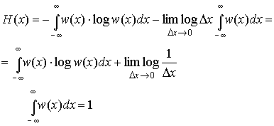
Второй
член в полученном выражении стремится
к
![]()
и
совершенно не зависит от распределения
вероятностей Х. Это означает, что
собственная информация любой непрерывной
случайной величины бесконечно велика.
Физический смысл такого результата
становиться понятным, если учесть, что
в конечном диапазоне непрерывная
величина может принимать бесконечное
множество значений, поэтому вероятность
того, что ее реализация будет точно
равна какому-то наперед заданному
конкретному значению является бесконечно
малой величиной 0. В результате энтропия,
определенная в соответствии с (1.4),
характеризующая среднюю степень
неожиданности появления возможных
реализаций для любой непрерывной
случайной величины не зависит от ее
закона распределения и всегда равна
бесконечности. Поэтому для описания
информационных свойств непрерывных
величин необходимо ввести другие
характеристики. Это можно сделать, если
обратить внимание на то, что первое
слагаемое выражении (3.34) является
конечным и однозначно определяется
плотностью распределения вероятности
w(x). Его называют дифференциальной
энтропией и обозначают h(x):
|
|
(3.35) |

Дифференциальная
энтропия обладает следующими свойствами.
1.
Дифференциальная энтропия в отличии
от обычной энтропии дискретного источника
не является мерой собственной информации,
содержащейся в ансамбле значений
случайной величины Х. Она зависит от
масштаба Х и может принимать отрицательные
значения. Информационный смысл имеет
не сама дифференциальная энтропия, а
разность двух дифференциальных энтропий,
чем и объясняется ее название.
2.
Дифференциальная энтропия не меняется
при изменении всех возможных значений
случайной величины Х на постоянную
величину. Действительно, масштаб Х при
этом не меняется и
справедливо равенство
|
|
(3.36) |
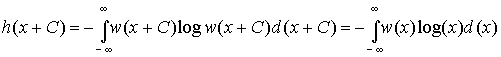
Из
этого следует, что h(x) не зависит от
математического ожидания случайной
величины, т.к. изменяя все значения Х на
С мы тем самым изменяем на С и ее среднее,
то есть математическое ожидание.
3.
Дифференциальная энтропия аддитивна,
то есть для объединения ХY независимых
случайный величин Х и Y справедливо:
h(XY)=
h(X)+ h(Y).
Доказательство этого свойства
аналогично доказательству (1.8) аддитивности
обычной энтропии.
4. Из всех
непрерывных величин Х с фиксированной
дисперсией 2
наибольшую дифференциальную энтропию
![]()
имеет
величина с гауссовским распределением,
т.е.
|
|
(3.37) |
Доказательство
свойства проведем в два этапа: сначала
вычислим h(x) для гауссовского распределения,
задаваемого плотностью.

где
м — математическое ожидание,
а затем
докажем неравенство (3.37).
Подставив
(3.38) в (3.35) найдем<

Для
доказательства неравенства (3.37) зададимся
произвольным распределением (х) с
дисперсией 2
и математическим ожиданием m и вычислим
интеграл J вида
|
|
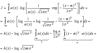
Но
в силу неравенства (1.7)
с учетом правила изменения основания
логарифмов (log t = log e ln t)
имеем:
|
|

|
|
так |

Таким
образом
![]()
,
откуда
![]()
.
Но
как только что было показано,
![]()
—
это дифференциальная энтропия гауссовского
распределения. Доказанное неравенство
и означает, что энтропия
гауссовского распределения
максимальна.
Попытаемся теперь
определить с помощью предельного
перехода взаимную
информацию между двумя непрерывными
случайными величинами X и Y. Разбив
области определения Х и Y соответственно
на небольшие интервалы x и y, заменим
эти величины дискретными так же, как
это делалось при выводе формулы
(3.34).
Исходя из выражения
(1.14) можно определить взаимную информацию
между величинами Х и Y .
|
|
(3.39) |

При
этом предельном переходе никаких явных
бесконечностей не появилось, т.е. взаимная
информация оказывается величиной
конечной, имеющей тот же смысл, что и
для дискретных сообщений.
С
учетом того, что
|
(x,y)= (y) |
равенство
(3.39) можно представить в виде
|
|
(3.40) |
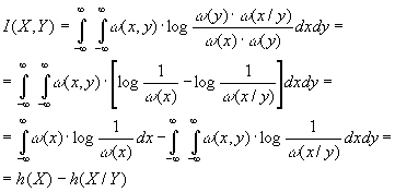
Здесь
h(X) — определенная выражением (3.35)
дифференциальная энтропия Х, а
|
|
(3.41) |
h(X/Y)
— условная дифференциальная энтропия.
Можно показать, что во всех случаях
h(X/Y)h(X).
Формула
(3.40) имеет ту же форму, что и (1.13), а
отличается лишь заменой энтропии
дифференциальной энтропией. Легко
убедиться, что основные свойства 1 и 2
(см. пункт 1.3) взаимной информации,
описываемые равенствами (1.15)(1.17),
остаются справедливыми и в этом случае.
3.4 -энтропия
и -производительность
источника непрерывных сообщений
Как
было показано в § 3.3, в одном отсчете
любого непрерывного сообщения содержится
бесконечное количество собственной
информации. И тем не менее, непрерывные
сообщения (телефонные разговоры,
телепередачи) успешно передаются по
каналам связи. Это объясняется тем, что
на практике никогда не требуется
абсолютно точного воспроизведения
переданного сообщения, а для передачи
даже с очень высокой, но ограниченной
точностью, требуется конечное количество
информации, также как и при передаче
дискретных сообщений. Данное обстоятельство
и положено в основу определения
количественной меры собственной
информации, источников непрерывных
сообщений. В качестве такой меры,
принимается минимальное количество
информации, необходимое для воспроизведения
непрерывного сообщения с заданной
точностью. Очевидно, что при таком
подходе собственная информация зависит
не только от свойств источника сообщений,
но и от выбора параметра , характеризующего
точность воспроизведения. Возможны
различные подходы к определению в
зависимости от вида и назначения
передаваемой информации. Наиболее часто
в информационной технике в качестве
используют среднеквадратическое
отклонение между принятым у и переданным
х сигналами, отражающими непрерывные
сообщения, т.е.
|
|
(3.42) |
где
Х и Y – ансамбли сигналов, отражающих
исходное и воспроизведенное сообщения.
Два
варианта сообщения или сигнала,
различающиеся не более, чем на заданное
значение 0,
называются эквивалентными. Взаимная
информация
I(X,Y) между двумя эквивалентными процессами
X(t) и Y(t) может быть определена в соответствии
с (3.40) как
|
I(X,Y)=h(X)-h(X/Y), |
где
h(X) и h(X/Y) – соответственно дифференциальная
и условная дифференциальная энтропии.
Из приведенного выражения видно,
что величина I(X,Y) зависит не только от
собственного распределения (х) ансамбля
Х (см. (3.35)), но и от условного распределения
(x/y) (см. (3.41)), которое определяется
способом преобразования процесса X в
Y. Для характеристики собственной
информации, содержащейся в одном отсчете
процесса Х, нужно устранить ее зависимость
от способа преобразования сообщения Х
в эквивалентное ему сообщение Y. Этого
можно добиться, если под количеством
собственной информации или — энтропией
H(Х)
процесса Х понимать минимизированную
по всем распределениям (X/Y) величину
I(X,Y), при которой сообщения Х
и Y еще эквивалентны, т.е.
|
|
(3.43) |
Таким
образом,
— энтропия
определяет минимальное количество
информации, содержащейся в одном отсчете
непрерывного
сообщения,
необходимое для воспроизведения его с
заданной верностью.
Если ансамбль
сообщений Х представляет собой процесс
с дискретным
временем
с непрерывными отсчетами, то под
— производительностью источника понимают
величину
|
|
(3.44) |
где
с
– количество отсчетов сообщения,
выдаваемых в единицу времени.
В том
случае, когда Х — непрерывный случайный
процесс с ограниченным спектром, вся
информация, содержащаяся в его значениях,
эквивалентна информации, содержащейся
в отсчетах процесса, следующих друг за
другом с интервалом
![]()
,
(fm-граничная
частота спектра), т.е. со
скоростью
|
c=2 |
(3.45) |
При
этом
— производительность
источника или процесса по-прежнему
определяется выражением (3.44), где величина
с
рассчитывается из условия (3.45).
В том
случае, если следующие друг за другом
отсчеты процесса коррелированны
(взаимозависимы), величина Н(Х)
в (3.43) должна вычисляться с учетом
вероятностных связей между отсчетами.
Итак,
— производительность источника
непрерывных сообщений представляет
собой минимальное количество информации,
которое нужно создать источнику в
единицу времени, для воспроизведения
его сообщений с заданной верностью.
— производительность называют также
скоростью создания информации при
заданном критерии верности.
Максимально
возможная — производительность
![]()
непрерывного
источника Х обеспечивается при гауссовском
распределении Х с дисперсией
![]()
(при
этом условии h(X) максимальна (см. (3.37)).
Оценим значение
.
Рассмотрим случай, когда непрерывное
сообщение X(t) представляет собой
стационарный гауссовский процесс с
равномерным энергетическим спектром,
ограниченным частотой Fc,
и с заданной мощностью (дисперсией) Рх,
а критерий эквивалентности задан в
виде (3.42).
Будем считать, что заданная верность
воспроизведения обусловлена действием
аддитивной статистически не связанной
с сигналом помехи (t) с математическим
ожиданием М[]=0 и дисперсией (мощностью)
![]()
.
Исходный сигнал Х рассматриваем
как сумму воспроизводящего сигнала Y и
помехи:
|
X=Y+. |
При
этом, поскольку (x/y)= (y+/y)= (/y)=
(), то h(X/Y) полностью определяется
шумом воспроизведения (t). Поэтому max
h(X/Y)=max h(). Так как шум воспроизведения
имеет фиксированную дисперсию
![]()
,
то дифференциальная энтропия имеет
максимум (3.37) при гауссовском
распределении шума
|
|
В
свою очередь дифференциальная энтропия
гауссовского источника с дисперсией
![]()
.
|
|
Следовательно,
— энтропия на один отсчет
сообщения
|
|
(3.46) |

Величина
![]()
характеризует
минимальное отношение сигнал-шум, при
котором сообщения X(t) и Y(t) еще
эквивалентны.
Согласно теореме
Котельникова
шаг
дискретизации
![]()
,
а c=2
Fc.
При этом равномерность спектра сообщения
обеспечивает некоррелированность
отстоящих на t друг от друга отсчетов,
а гауссовский характер распределения
X(t) — их независимость. Следовательно,
в соответствии с (3.44)
|
|
или с учетом (3.46)
|
|
(3.47) |
Количество
информации,
выданное таким источником за время Тс
|
|
(3.48) |
Интересно
отметить, что правая часть выражения
(3.48) совпадает с наиболее общей
характеристикой сигнала, называемой
его объемом, если принять динамический
диапазон сигнала D=log
0.
Это означает, что объем сигнала равен
максимальному количеству информации,
которое может содержаться в сигнале
длительностью Тс.
Соседние файлы в предмете [НЕСОРТИРОВАННОЕ]
- #
- #
- #
- #
- #
- #
- #
- #
- #
- #
- #
Макеты страниц
3.9.1. Общие сведения
В данном параграфе предпотагается, что:
а) входной сигнал  нормирован в соответствии

б) разрядность входного сигнала (АЦП) после запятой равна 
в) разрядности (после запятой) всех регистров умножителей и сумматоров ЦФ равны 
г) при квантовании используется округление.
3.9.2. Детерминированные оценки
Детерминированные оценки определяют абсолютные границы (диапазон изменения) ошибок квантования выходного сигнала в ЦФ и получаются с использованием линейной модели ЦФ (см. 3.8) на основе оценок ошибок квантования сигналов при выполнении элементарных операций, определяемых (3.18) — (3.20).
Ошибка квантования входного сигнала

Ошибка квантования сигнала на выходах умножителей

Эквивалентная ошибка квантования на выходе сумматора ЦФ

где  — число умножителей, подключенных к
  сумматору.
Составляющая выходной ошибки квантования, обусловленная квантованием входного сигнала,

Составляющая выходной ошибки квантования, обусловленная квантованием сигналов на выходах умножителей, подключенных к  сумматору,

Ошибка квантования выходного сигнала (с учетом 

Пример 3.20. Рассматривается каскадная структура РЦФ восьмого порядка с передаточной функцией  при прямой форме реализации элементарных звеньев второго порядка (см. рис. 3.5, в), где
Шумовой сигнал  проходит на выход через весь фильтр с передаточной функцией
  а сигналы
  части фильтра с передаточными функциями:
  соответственно (см. рис. 3.5, в и 3.8). Для получения оценки ошибки квантования на ЭВМ рассчитываются величины
  Эти величины равны:
Тогда из (3.21) и (3.22) получаем оценки составляющих выходного шума; 
Оценка ошибки квантования выходного сигнала определяется из (3.23) с Учетом (3.18) и (3.19):

3.9.3. Вероятностные оценки
Вероятностные оценки шума квантования выходного сигнала основаны на представлении ошибок квантования сигналов при выполнении элементарные операций как случайных шумоподобных процессов типа «белый шум» (см. 3.6) причем считается, что любые два источника шума создают некоррелированные шумы [3.3]. При получении оценок используется линейная модель ЦФ (см 3.8).
Дисперсия шума квантования входного сигнала

Дисперсия шума квантования сигнала на выходах умножителей

Дисперсия эквивалентного шума квантования на выходе сумматора ЦФ

где  — число умножителей, подключенных к
  сумматору.
Дисперсия составляющей выходного шума, обусловленной квантованием входного сигнала,

Дисперсия составляющей выходного шума, обусловленной квантованием сигналов на выходах умножителей, подключенных к  сумматору,

Дисперсия выходного шума квантования [с учетом (3.24) — (3.28)]

В ряде случаев (как правило, для  вычисления по
  можно упростить, применив для вычисления бесконечных сумм квадратов отсчетов ипульсных характеристик формулы:

Вычисления по (3.30) и (3.31) можно выполнить численными методами на ЭВМ или оценить по графику функции квадрата  Вычисления по
  выполняются с помощью теоремы о вычетах [3.4].
При произвольной спектральной плотности мощности  входного шума дисперсия составляющей выходного шума, обусловленная квантованием входного сигнала, может быть вычислена по формулам:

где  — спектральная плотность мощности выходного шума.
Пример 3.21. Рассматривается РЦФ первого порядка с передаточной функцией  Шумовой сигнал
  проходит на выход через весь фильтр с передаточной функцией
  и импульсной характеристикой
  а сигнал
  определяемый шумами двух умножителей, подключенных к сумматору, — через часть фильтра с передаточной функцией
  и импульсной характеристикой
  Используя (3.29), получаем

Аналогичный результат получается при использовании формул  (см. пример 2.16).
Пример 3.22. Рассматривается равнололосный НЦФ с передаточной функцией  где
где  (см. пример 4.9). Линейная модель ЦФ показана на рис. 3.7.
Амплитудно-частотная характеристика фильтра  аппроксимирует характеристику, показанную на рис. 3.9 (кривая
Здесь же показан вид квадрата аппроксимируемой АЧХ (кривая 2).
Для оценки суммы квадратов отсчетов импульсной характеристики воспользуемся (3.30) и рис. 3.9 (т. е. вычислим площадь под кривой 2). Оценка составляющей

Отметим, что полученная оценка близка к значению дисперсии, рассчитанной по заданным коэффициентам  с помощью формулы (3.27):

Учитывая, что только девять коэффициентов  отличны от 0 (т. е. шум

Рис. 3.9
округления образуется на выходах девятя умножителей), по формуле (3.29) получаем оценку дисперсии выходного шума

Ошибка квантования
- Ошибка квантования
-
Шум квантования — ошибки, возникающие при оцифровке аналогового сигнала. В зависимости от типа аналого-цифрового преобразования могут возникать из-за округления (до определённого разряда) сигнала или усечения (отбрасывания младших разрядов) сигнала.
Содержание
- 1 Математическое описание
- 1.1 Модель
- 1.2 Детерминированные оценки
- 1.3 Вероятностные оценки
- 2 См. также
- 3 Ссылки
Математическое описание
Модель
Шум квантования можно представить как аддитивный дискретный сигнал
 , учитывающий ошибки квантования. Если — входной сигнал квантователя, а — его передаточная функция, то имеем следующую линейную модель шума квантования:
Линейная модель используется для аналитического исследования свойств шума квантования.
Детерминированные оценки
Детерминированные оценки позволяют определить абсолютные границы шума квантования:
- ,
где
— число разрядов квантования (сигнала ), — шаг квантования — при округлении — при усечении.Вероятностные оценки
Вероятностные оценки основаны на представлении ошибок квантования (сигнала e(nT)) как случайного шумоподобного процесса. Допущения, вводимые относительно шума квантования:
В таком случае математическое ожидание
и дисперсия шума квантования определяется следующим образом (при квантовании используется дополнительный код):См. также
- Отношение сигнал-шум
- Дизеринг
Ссылки
- Round-Off Error Variance(англ.)
- «Цифровая обработка сигналов». Л. М. Гольденберг, Б. Д. Матюшкин — М.: Радио и связь, 1985
- 1 Математическое описание
 , учитывающий ошибки квантования. Если
  — входной сигнал квантователя, а
 ![F[] !](https://dic.academic.ru/pictures/wiki/files/100/d9a67617bcc2874e5dcee5df989f5f52.png) — его передаточная функция, то имеем следующую линейную модель шума квантования:
— его передаточная функция, то имеем следующую линейную модель шума квантования:![e(nT) = F[d(nT)] - d(nT) !](https://dic.academic.ru/pictures/wiki/files/48/0bf1032d4991203805b67afcb4832b06.png)
![|max[e(nT)]| = frac{1}{m} 2^{-b} = frac{1}{m} Q](https://dic.academic.ru/pictures/wiki/files/97/a2a6cf1f23b3dd15c4169c59cd1338f4.png) ,
, — число разрядов квантования (сигнала
  — шаг квантования
  — при округлении
  — при усечении.
 и дисперсия
  шума квантования определяется следующим образом (при квантовании используется дополнительный код):
 Wikimedia Foundation.
2010.
Полезное
Смотреть что такое «Ошибка квантования» в других словарях:
-
ошибка квантования — Ошибка, вызванная несоответствием формы выходного (квантованного) и входного (аналогового) сигналов. Зависит от величины шага квантования и частоты дискретизации. [Л.М. Невдяев. Телекоммуникационные технологии. Англо русский толковый словарь… … Справочник технического переводчика
-
ошибка квантования — kvantavimo paklaida statusas T sritis automatika atitikmenys: angl. quantization error vok. Quantisierungsfehler, m rus. ошибка квантования, f pranc. erreur de quantification, f … Automatikos terminų žodynas
-
ошибка округления — погрешность, возникающая при квантовании в результате округления амплитуды сигнала до ближайшего уровня квантования. Причина возникновения шума квантования … Русский индекс к Англо-русскому словарь по музыкальной терминологии
-
Аналого-цифровой преобразователь — Четырёхканальный аналого цифровой преобразователь Аналого цифровой преобразователь[1][2] … Википедия
-
АЦП — Четырёхканальный аналого цифровой преобразователь Аналого цифровой преобразователь (АЦП, ADC) устройство, преобразующее входной аналоговый сигнал в дискретный код (цифровой сигнал). Обратное преобразование осуществляется при помощи ЦАП (DAC)… … Википедия
-
Цифро-аналоговое преобразование — Четырёхканальный аналого цифровой преобразователь Аналого цифровой преобразователь (АЦП, ADC) устройство, преобразующее входной аналоговый сигнал в дискретный код (цифровой сигнал). Обратное преобразование осуществляется при помощи ЦАП (DAC)… … Википедия
-
шум дробления — Разновидность шума квантования, возникающего при аналого цифровом преобразовании сигнала малого уровня, когда ошибка квантования для разных отсчетов становится не равновероятной. Эффективной мерой снижения шума дробления является использование… … Справочник технического переводчика
-
Quantisierungsfehler — kvantavimo paklaida statusas T sritis automatika atitikmenys: angl. quantization error vok. Quantisierungsfehler, m rus. ошибка квантования, f pranc. erreur de quantification, f … Automatikos terminų žodynas
-
erreur de quantification — kvantavimo paklaida statusas T sritis automatika atitikmenys: angl. quantization error vok. Quantisierungsfehler, m rus. ошибка квантования, f pranc. erreur de quantification, f … Automatikos terminų žodynas
-
kvantavimo paklaida — statusas T sritis automatika atitikmenys: angl. quantization error vok. Quantisierungsfehler, m rus. ошибка квантования, f pranc. erreur de quantification, f … Automatikos terminų žodynas
Digital Filters
Marcio G. Siqueira, Paulo S.R. Diniz, in The Electrical Engineering Handbook, 2005
2.11 Quantization in Digital Filters
Quantization errors in digital filters can be classified as:
- •
-
Round-off errors derived from internal signals that are quantized before or after more down additions;
- •
-
Deviations in the filter response due to finite word length representation of multiplier coefficients; and
- •
-
Errors due to representation of the input signal with a set of discrete levels.
A general, digital filter structure with quantizers before delay elements can be represented as in Figure 2.23, with the quantizers implementing rounding for the granular quantization and saturation arithmetic for the overflow nonlinearity.

FIGURE 2.23. Digital Filter Including Quantizers at the Delay Inputs
The criterion to choose a digital filter structure for a given application entails evaluating known structures with respect to the effects of finite word length arithmetic and choosing the most suitable one.
2.11.1 Coefficient Quantization
Approximations are known to generate digital filter coefficients with high accuracy. After coefficient quantization, the frequency response of the realized digital filter will deviate from the ideal response and eventually fail to meet the prescribed specifications. Because the sensitivity of the filter response to coefficient quantization varies with the structure, the development of low-sensitivity digital filter realizations has raised significant interest (Antoniou, 1993; Diniz et al., 2002).
A common procedure is to design the digital filter with infinite coefficient word length satisfying tighter specifications than required, to quantize the coefficients, and to check if the prescribed specifications are still met.
2.11.2 Quantization Noise
In fixed-point arithmetic, a number with a modulus less than one can be represented as follows:
(2.84)x=b0b1b2b3…bb,
where b0 is the sign bit and where b1b2b3 … bb represent the modulus using a binary code. For digital filtering, the most widely used binary code is the two’s complement representation, where for positive numbers b0 = 0 and for negative numbers b0 = 1. The fractionary part of the number, called x2 here, is represented as:
(2.85)x2={xif b0=0.2−|x|if b0=1.
The discussion here concentrates in the fixed-point implementation.
A finite word length multiplier can be modeled in terms of an ideal multiplier followed by a single noise source e(n) as shown in Figure 2.24.

FIGURE 2.24. Model for the Noise Generated after a Multiplication
For product quantization performed by rounding and for signal levels throughout the filter much larger than the quantization step q = 2−b, it can be shown that the power spectral density of the noise source ei(n) is given by:
(2.86)Pei(z)=q212=2−2b12.
In this case, ei(n) represents a zero mean white noise process. We can consider that in practice, ei(n) and ek(n + l) are statistically independent for any value of n or l (for i ≠ k). As a result, the contributions of different noise sources can be taken into consideration separately by using the principle of superposition.
The power spectral density of the output noise, in a fixed-point digital-filter implementation, is given by:
(2.87)Py(z)=σe2Σi=1KGi(z)Gi(z−1),
where Pei(ejw)=σe2, for all i, and each Gi(z) is a transfer function from multiplier output (gi(n)) to the output of the filter as shown in Figure 2.25. The word length, including sign, is b + 1 bits, and K is the number of multipliers of the filter.

FIGURE 2.25. Digital Filter Including Scaling and Noise Transfer Functions.
2.11.3 Overflow Limit Cycles
Overflow nonlinearities influence the most significant bits of the signal and cause severe distortion. An overflow can give rise to self-sustained, high-amplitude oscillations known as overflow limit cycles. Digital filters, which are free of zero-input limit cycles, are also free of overflow oscillations if the overflow nonlinearities are implemented with saturation arithmetic, that is, by replacing the number in overflow by a number with the same sign and with maximum magnitude that fits the available wordlength.
When there is an input signal applied to a digital filter, overflow might occur. As a result, input signal scaling is required to reduce the probability of overflow to an acceptable level. Ideally, signal scaling should be applied to ensure that the probability of overflow is the same at each internal node of the digital filter. This way, the signal-to-noise ratio is maximized in fixed-point implementations.
In two’s complement arithmetic, the addition of more than two numbers will be correct independently of the order in which they are added even if overflow occurs in a partial summation as long as the overall sum is within the available range to represent the numbers. As a result, a simplified scaling technique can be used where only the multiplier inputs require scaling. To perform scaling, a multiplier is used at the input of the filter section as illustrated in Figure 2.25.
It is possible to show that the signal at the multiplier input is given by:
(2.88)xi(n)=12πj∮cXi(z)zn−1dz=12π∫02πFi(ejω)X(ejω)ejωndω,
where c is the convergence region common to Fi(z) and X(z).
The constant λ is usually calculated by using Lp norm of the transfer function from the filter input to the multiplier input Fi(z), depending on the known properties of the input signal. The Lp norm of Fi(z) is defined as:
(2.89)‖Fi(ejω)‖p=[12π∫02π|Fi(ejω)|pdω]1p,
for each p ≥ 1, such that ∫02π|Fi(ejω)|pdω≤∞. In general, the following inequality is valid:
(2.90)|xi(n)| ≤ ‖Fi‖p‖X‖q, (1p+1q=1),
for p, q = 1, 2 and ∞.
The scaling guarantees that the magnitudes of multiplier inputs are bounded by a number Mmax when |x(n)| ≤ Mmax. Then, to ensure that all multiplier inputs are bounded by Mmax we must choose λ as follows:
(2.91)λ=1Max{‖F1‖p,…,‖F1‖p,…, ‖FK‖p},
which means that:
(2.92)‖F′i(ejω)‖p≤1, for‖X(ejω)‖q ≤ Mmax.
The K is the number of multipliers in the filter.
The norm p is usually chosen to be infinity or 2. The L∞ norm is used for input signals that have some dominating frequency component, whereas the L2 norm is more suitable for a random input signal. Scaling coefficients can be implemented by simple shift operations provided they satisfy the overflow constraints.
In case of modular realizations, such as cascade or parallel realizations of digital filters, optimum scaling is accomplished by applying one scaling multiplier per section.
As an illustration, we present the equation to compute the scaling factor for the cascade realization with direct-form second-order sections:
(2.93)λi=1‖∏j=1i−1Hj(z)Fi(z)‖p,
where:
Fi(z)=1z2+m1iz+m2i.
The noise power spectral density is computed as:
(2.94)Py(z)=σe2[3+3λ12∏i=1mHi(z)Hi(z−1)+5Σj=2m1λj2∏i=jmHi(z)Hi(z−1)],
whereas the output noise variance is given by:
(2.95)σo2=σe2[3+3λ12||∏i=1mHi(ejω)||22+5Σj=2m1λj2||∏i=jmHi(ejω)||22].
As a design rule, the pairing of poles and zeros is performed as explained here: poles closer to the unit circle pair with closer zeros to themselves, such that ||Hi(z)||p is minimized for p = 2 or p = ∞.
For ordering, we define the following:
(2.96)Pi=| |Hi(z)| |∞| |Hi(z)| |2.
For L2 scaling, we order the section such that Pi is decreasing. For L∞ scaling, Pi should be increasing.
2.11.4 Granularity Limit Cycles
The quantization noise signals become highly correlated from sample to sample and from source to source when signal levels in a digital filter become constant or very low, at least for short periods of time. This correlation can cause autonomous oscillations called granularity limit cycles.
In recursive digital filters implemented with rounding, magnitude truncation,72 and other types of quantization, limitcycles oscillations might occur.
In many applications, the presence of limit cycles can be harmful. Therefore, it is desirable to eliminate limit cycles or to keep their amplitude bounds low.
If magnitude truncation is used to quantize particular signals in some filter structures, it can be shown that it is possible to eliminate zero-input limit cycles. As a consequence, these digital filters are free of overflow limit cycles when overflow nonlinearities, such as saturation arithmetic, are used.
In general, the referred methodology can be applied to the following class of structures:
- •
-
State-space structures: Cascade and parallel realization of second-order state-space structures includes design constraints to control nonlinear oscillations (Diniz and Antoniou, 1986).
- •
-
Wave digital filters: These filters emulate doubly terminated lossless filters and have inherent stability under linear conditions as well as in the nonlinear case where the signals are subjected to quantization (Fettweis, 1986).
- •
-
Lattice realization: Modular structures allowing easy limit cycles elimination (Gray and Markel, 1975).
Read full chapter
URL:
https://www.sciencedirect.com/science/article/pii/B9780121709600500621
Biomedical signals and systems
Sri Krishnan, in Biomedical Signal Analysis for Connected Healthcare, 2021
2.2.1 Noise power
The quantization error (e) or noise tends to have a random behavior, and they could be mathematically represented using statistical variables. Power of a random variable with a probability density function of p(e) could be obtained by computing the second-order statistics of variance, and it is denoted by
σ2=∫−q/2q/2e2p(e)de
A good assumption for p(e) is a uniform probability density function which will have a value of 1/q over the range of −q/2 to q/2.
=∫−q/2q/2e2·1qde=q212
Read full chapter
URL:
https://www.sciencedirect.com/science/article/pii/B9780128130865000049
Measurement of high voltages
E. Kuffel, … J. Kuffel, in High Voltage Engineering Fundamentals (Second Edition), 2000
Static errors
The quantization error is present because the analogue value of each sample is transformed into a digital word. This A-to-D conversion entails a quantization of the recorder’s measuring range into a number of bands or code bins, each represented by its central value which corresponds to a particular digital code or level. The number of bands is given by 2N, where N is the resolution of the A-to-D converter. The digital output to analogue input relationship of an ideal digitizer is shown diagrammatically in Fig. 3.49. For any input in the range (iΔVav – 0.5 * ΔVav to iΔVav + 0.5 * ΔVav), where iΔVav is the voltage corresponding to the width of each code bin, or one least significant bit (LSB), and iΔVav is the centre voltage corresponding to the i th code, an ideal digitizer will return a value of Ii. Therefore, the response of an ideal digitizer to a slowly increasing linear ramp would be a stairway such as that shown in Fig. 3.50. A quick study of these figures reveals the character of the quantization error associated with the ideal A-to-D conversion process. The maximum error possible is equivalent to a voltage corresponding to ±(½) of an LSB. For an ideal digital recorder, this quantization would be the only source of error in the recorded samples. For a real digital recorder, this error sets the absolute upper limit on the accuracy of the readings. In the case of an 8-bit machine, this upper limit would be 0.39 per cent of the recorder’s full-scale deflection. The corresponding maximum accuracy (lowest uncertainty) of a 10-bit recorder is 0.10 per cent of its full-scale deflection.

Figure 3.49. Analogue input to digital output relation of an ideal A/D converter

Figure 3.50. Response of an ideal A/D converter to a slowly rising ramp
The error caused by discrete time sampling is most easily demonstrated with reference to the recording of sinusoidal signals. As an example we can look at the discrete time sampling error introduced in the measurement of a single cycle of a pure sine wave of frequency f, which is sampled at a rate of four times its frequency. When the sinusoid and the sampling clock are in phase, as shown in Fig. 3.51, a sample will fall on the peak value of both positive and negative half-cycles. The next closest samples will lie at π/2 radians from the peaks. As the phase of the clock is advanced relative to the input sinusoid the sample points which used to lie at the peak values will move to lower amplitude values giving an error (Δ) in the measurement of the amplitude (A) of

Figure 3.51. Sample points with sinusoid and sampling clock in phase. (Error in peak amplitude = 0)
Δ = A(1 − cos ϕ)
where ϕ is the phase shift in the sample points. This error will increase until ϕ – π/4 (Fig. 3.52). For ϕ > π/4 the point behind the peak value will now be closer to the peak and the error will decrease for a ϕ in the range of π/4 to π/2. The maximum per unit value of the discrete time sampling error is given by eqn 3.93,

Figure 3.52. Sample points with sampling clock phase advanced to π/4 with respect to the sinusoid. Error in peak amplitude (Δ) is at a maximum
(3.93)Δmax=I−cos(πfts)
where ts is the recorder’s sampling interval and f the sinewave frequency.
The maximum errors obtained through quantization and sampling when recording a sinusoidal waveform are shown in Fig. 3.53. The plotted quantities were calculated for an 8-bit 200-MHz digitizer.

Figure 3.53. Sampling and quantization errors of an ideal recorder
In a real digital recorder, an additional two categories of errors are introduced. The first includes the instrument’s systematic errors. These are generally due to the digitizer’s analogue input circuitry, and are present to some degree in all recording instruments. They include such errors as gain drift, linearity errors, offset errors, etc. They can be compensated by regular calibration without any net loss in accuracy. The second category contains the digitizer’s dynamic errors. These become important when recording high-frequency or fast transient signals. The dynamic errors are often random in nature, and cannot be dealt with as simply as their systematic counterparts and are discussed below.
Read full chapter
URL:
https://www.sciencedirect.com/science/article/pii/B9780750636346500046
Remaining useful life prediction
Yaguo Lei, in Intelligent Fault Diagnosis and Remaining Useful Life Prediction of Rotating Machinery, 2017
6.3.4.3 RUL Prediction
The constructed indicator WMQE is further input into the RUL prediction module. In this module, a PF-based prediction algorithm is utilized to predict RUL of the rotating machinery whose degradation processes are described using a variant of Paris–Erdogan model. The Paris–Erdogan model is formulated as
(6.96)dxdt=c(Δδ)γ, Δδ=mx
where x represents the semicrack length, t is the number of stress cycles (i.e., the fatigue life), c, γ, and m are material constants which are determined by tests, and Δδ is amplitude of stress intensity factor roughly proportional to the square root of x.
It is seen from Eq. (6.96) that there are several model parameters in the Paris–Erdogan model, that is, c, γ, and m, which are difficult to measure during the operation process of the rotating machinery. For convenient application, the Paris–Erdogan model is transformed into the following format with α=cmγ and β = γ/2.
(6.97)dxdt=αxβ.
Then, the above function is rewritten into the following state space model.
(6.98)xk=xk−1+αk−1xk−1βΔtkαk=αk−1zk=xk+νk,
where αk−1 is a random variable following a normal distribution of Nμα,σα2, β is a constant parameter, Δtk=tk−tk−1, zk is the measured WMQE value at tk and νk is the measurement noise following the normal distribution of N0,σν2. With the transformation of the Paris–Erdogan model, the model parameters are more convenient to estimate according to the measurements. In addition, the state space model inherits the superiority of the Paris–Erdogan model in describing the general degradation processes. Therefore, it is supposed to be a good model for a general degradation process.
After the transformation, the unknown model parameters are changed to be Θ=μα,σα2,β,σν2′, where (·)′ denotes the vector transposition. Then, the measured WMQE values constructed from vibration signals are input into the model, and the model parameters are initialized using MLE. It is assumed that there are a series of measurements z0:M=z0,…,zM′ at ordered times t0,…,tM. According to Eq. (6.98), zk is formulated as follows:
(6.99)zk=xk−1+αkxk−1βΔtk+νk.
The degradation state xk−1 has the following relationship with the measurement zk−1.
(6.100)xk−1=zk−1−νk−1.
The degradation state xk−1 is hard to be acquired in real applications. If the measurement noise νk−1 is small enough compared with the measurement itself, it is negligible and xk−1 is approximated by zk−1. Let T=z0βΔt1,…,zM−1βΔtM′. z1:M=z1,…,zM′ is multivariate normally distributed, which is denoted as follows:
(6.101)z1:M∼Nz0:M−1+μαT,σα2TT′+σν2IM,
where IM is an identity matrix of order M.
Let Δz1:M=z1−z0,…,zM−zM−1′, and the log-likelihood function of the unknown parameters based on the measurements is expressed as
(6.102)ℓΘ|z0:M=−M2ln2π−12lnσα2TT′+σν2IM −12Δz1:M−μαT′σα2TT′+σν2IM−1Δz1:M−μαT =−M2ln2π−M2lnσα2−12lnTT′+σ˜ν2IM −12σα2Δz1:M−μαT′σα2TT′+σν2IM−1Δz1:M−μαT,
with σ~ν2=σν2/σα2. The first partial derivatives of ℓΘ|z0:M with respect to μα and σα2 are calculated and formulated with
(6.103)∂ℓΘ|z0:M∂μα=1σα2T′TT′+σ~ν2IM-1Δz1:M−μαT,
(6.104)∂ℓΘ|z0:M∂σα2=−M2σα2+12σα4Δz1:M−μαT′TT′+σ~ν2IM−1Δz1:M−μαT.
Let ∂ℓΘ|z0:M/∂μα=0 and ∂ℓΘ|z0:M/∂σα2=0. The MLE results of μα and σα2 are
(6.105)μα=T′TT′+σ~ν2IM−1Δz1:MT′TT′+σ~ν2IM−1T,
(6.106)σα2=Δz1:M−μαT′TT′+σ~ν2IM−1Δz1:M−μαTM.
With Eqs. (6.105) and (6.106) substituted into Eq. (6.102), the log-likelihood function is reduced into a two-variable function about β and σ~ν2, which is denoted by
(6.107)ℓΘ|z0:M=−M2ln2π−M2lnσα2−12lnTT′+σ~ν2IM−M2.
The MLE values of β and σ~ν2 are obtained by maximizing the log-likelihood function (6.107) through two-dimensional optimizing. Then the MLE values of β and σ~ν2 are substituted into Eqs. (6.105) and (6.106), and the MLE values of μα and σα2 are acquired. The value of σν2 is calculated with σ~ν2 multiplied by σα2. Finally, all of the unknown parameters Θ=μα,σα2,β,σν2′ are initialized.
After parameter initialization, the model parameters are further updated and the RUL is predicted using a PF-based prediction algorithm. Based on the initialized parameters, a series of initial particles y0nn=1:Ns are sampled from the initial PDF of the system state p(y0n|Θ0)∼N(y0,Q0) with
(6.108)y0=x0μα and Q0=000σα2.
Ns is the number of particles and the weight of each particle is set to be 1/Ns. Then new particles ykni=1:Ns are obtained following
(6.109)ykn=xknμαn=xk−1n+μαnxk−1nβΔtkμαn.
When the new measurement zk at tk is available, each particle weight is updated and normalized by
(6.110)wkn=wk−1npzk|ykn, w~kn=wkn∑n=1Nswkn,
where
(6.111)pzk|ykn=12πσνexp−12zk−xknσν2.
The particles are resampled according to the particle weights and their weights are reset to be 1/Ns. After that, the RUL is predicted based on the resampled particles. The RUL lk at tk is defined as
(6.112)lk=inflk:xlk+tk≥λ|x1:k,
where λ is a prespecified failure threshold. Each particle is transmitted following the transition function of Eq. (6.98) from current state until the state value exceeds the failure threshold, and the RUL lknn=1:Ns predicted using each particle is acquired. Then the PDF of the RUL is approximated by
(6.113)plk|z0:k=∑n=1Nsw~knδlk−lkn.
Read full chapter
URL:
https://www.sciencedirect.com/science/article/pii/B9780128115343000068
Orbit and Attitude Sensors
Enrico Canuto, … Carlos Perez Montenegro, in Spacecraft Dynamics and Control, 2018
Exercise 1
Prove that the quantization error defined by Eq. (8.6) is bounded by |n˜y(i)|≤ρy/2 and under the random assumption has zero mean and variance equal to ρy2/12. □
A typical model of the random error d˜ in Eq. (8.4), which includes quantization errors, is the linear continuous-time stochastic state equation
(8.7)x˜˙(t)=A˜x˜+G˜w˜d˜(t)=C˜x˜+D˜w˜E{w˜(t)}=0,E{w˜(t)w˜T(t+τ)}=S˜w2δ(τ)E{x˜(0)}=x˜0,E{(x˜(0)−x˜0)(x˜(0)−x˜0)T}=P˜0≥0E{(x˜(0)−x˜0)w˜T(0)}=0,
which is similar to the DT Eq. (4.159) of Section 4.8.1. Eq. (8.7) being continuous-time, the eigenvalues of the state matrix A˜ are assumed to lie on the imaginary axis and when equal to zero may be multiple. The statistics in Eq. (8.7) assumes that w˜ is a zero-mean second-order stationary white noise with constant spectral density S˜w2, and impulsive covariance, where δ(τ) denotes a Dirac delta (see Sections 13.2.1 and 13.7.3Section 13.2.1Section 13.7.3). The initial state may be modeled as a random vector with mean value x˜0 and covariance matrix P˜0, but is uncorrelated from any simultaneous white noise as expressed by the last identity in Eq. (8.7). This uncorrelation has been already referred to as the causality constraint. In principle, Eq. (8.7) may be unobservable from the output d˜ and uncontrollable by the noise w˜, because the output d˜ may include polynomial and trigonometric components (deterministic signals) just driven by the initial state x˜0. For instance, a trigonometric component tuned to the angular frequency ω˜ corresponds to a second-order subsystem with eigenvalues ±jω˜. A first-order polynomial corresponds to a second-order subsystem with a pair of zero eigenvalues and a single eigenvector. The mixed case of stochastic processes and deterministic signals can be simplified by assuming that trigonometric and polynomial components are the free response of the equations driven by w˜, and that Eq. (8.7) is observable and controllable.
The simplest model of the class in Eq. (8.7), which is common to inertial sensors (accelerometers in Section 8.4 and gyroscopes in Section 8.5), is the scalar first-order random drift [32]:
(8.8)x˜˙(t)=w˜x,x˜(0)=x˜0d˜(t)=x˜+w˜dE{x˜(0)}=x˜0,var{x˜}=σ02,E{(x˜−x˜0)w˜T(0)}=0w˜=[w˜xw˜d],E{w˜(t)}=0,E{w˜(t)w˜T(t+τ)}=[S˜wx200S˜wd2]δ(τ),
where, if [unit] denotes the unit of measurement of x˜, we find S˜wx2 in [(unit/s)2Hz−1] and S˜wd2 in [unit2Hz−1]. The initial state x˜0 accounts for a constant bias and is uncorrelated with any simultaneous noise; the scalar input noise w˜x and the output noise w˜d in Eq. (8.8) are uncorrelated with each other. The output process d˜ is nonstationary and the autocorrelation is given by
(8.9)R˜d(t,t+τ)=S˜wx2min(t,t+τ)+S˜wd2δ(τ).
Although x˜ is nonstationary, the spectral density S˜x2(f) can be defined through the AS equation x˜˙=−εx˜+w˜x, where ε > 0 must be sufficiently smaller than the cutoff frequency f0 to be defined in the next paragraph. We can write the following identities:
(8.10)S˜d2(f)=S˜x2(f)+S˜wd2=S˜wx2(2πf)2+S˜wd2,f>ε2π=fεσ˜x2=limf→∞∫0fS˜x2νdν<∞,
where if, for f < ε, S˜x2(f) is bounded, also the variance σ˜x2 is bounded. The Bode plot of S˜d(f) is approximately flat for f>f0=2π−1S˜wx/S˜wd>fε and has a −20 dB/decade slope for fε < f < f0. The first PSD in the first row of Eq. (8.10) is a first-order random walk, which is known, in the realm of inertial sensors, as the (long-term) bias instability of the sensor. The name is appropriate because it describes the long-term fluctuations—bounded because of ε—around the mean sensor bias x˜0. The square root of the second term S˜wd corresponds to the minimum-valued profile of the overall spectral density. Let us call it, as already anticipated, noise floor, although the name sometimes refers to the whole instrument noise (here referred to as the background noise). In the realm of inertial sensors, it is known as the velocity random walk in the case of linear accelerometers, the unit being [m/(s2Hz)], and the angular random walk (ARW) in the case of gyroscopes, the unit being[rad/(sHz)]. The name, which may cause same confusion, is justified by the fact that when either of the two measurements (linear acceleration and angular rate) is time integrated for generating either velocity or attitude measurements, the integrated noise floor becomes a random walk. By restricting to gyroscopes, the ARW unit [rad/(sHz)] is usually simplified to [rad/s], de facto to the non-SI unit [degree/hour]. Indeed, the simplified unit is at the same time the unit of S˜wd and the unit of the root mean square (RMS) σ¯w(t,Δt) of the random walk increment w¯d(t,Δt)=∫tt+Δtw˜d(τ)dτ, namely:
(8.11)σ¯w(t,Δt)=E{1Δt(∫tt+Δtw˜d(τ)dτ)2}=S˜wd.
Read full chapter
URL:
https://www.sciencedirect.com/science/article/pii/B9780081007006000088
Sampling Theory
Luis Chaparro, in Signals and Systems Using MATLAB (Second Edition), 2015
8.3.2 Quantization and Coding
Amplitude discretization of the sampled signal xs(t) is accomplished by a quantizer consisting of a number of fixed amplitude levels against which the sample amplitudes {x(nTs)} are compared. The output of the quantizer is one of the fixed amplitude levels that best represents {x(nTs)} according to some approximation scheme. The quantizer is a non-linear system.
Independent of how many levels or, equivalently, of how many bits are allocated to represent each level of the quantizer, in general there is a possible error in the representation of each sample. This is called the quantization error. To illustrate this, consider the 2-bit or four-level quantizer shown in Figure 8.12. The input of the quantizer are the samples {x(nTs)}, which are compared with the values in the bins [-2Δ,-Δ],[-Δ,0],[0,Δ], and [Δ,2Δ]. Depending on which of these bins the sample falls in it is replaced by the corresponding levels -2Δ,-Δ,0, or Δ, respectively. The value of the quantization step Δ for the four-level quantizer is

Figure 8.12. Four-level quantizer and coder.
(8.23)Δ=dynamic range of signal2b=2max|x(t)|22
where b = 2 is number of bits of the code assigned to each level. The bits assigned to each of the levels uniquely represents the different levels [-2Δ,-Δ,0,Δ]. As to how to approximate the given sample to one of these levels, it can be done by rounding or by truncating. The quantizer shown in Figure 8.12 approximates by truncation, i.e., if the sample kΔ≤x(nTs)<(k+1)Δ, for k = −2, −1,0,1, then it is approximated by the level kΔ.
To see how quantization and coding are done, and how to obtain the quantization error, let the sampled signal be
x(nTs)=x(t)|t=nTS
The given four-level quantizer is such that if the sample x(nTs) is such that
(8.24)kΔ≤x(nTs)<(k+1)Δ⇒xˆ(nTs)=kΔk=-2,-1,0,1
The sampled signal x(nTs) is the input of the quantizer and the quantized signal xˆ(nTs) is its output. So that whenever
-2Δ≤x(nTs)<-Δ⇒xˆ(nTs)=-2Δ-Δ≤x(nTs)<0⇒xˆ(nTs)=-Δ0≤x(nTs)<Δ⇒xˆ(nTs)=0Δ≤x(nTs)<2Δ⇒xˆ(nTs)=Δ
To transform the quantized values into unique binary 2-bit values, one could use a code such as
xˆ(nTs)⇒binary code-2Δ10-Δ110Δ00Δ01
which assigns a unique 2 bit binary number to each of the 4 quantization levels. Notice that the first bit of this code can be considered a sign bit, “1” for negative levels and “0” for positive levels.
If we define the quantization error as
ε(nTs)=x(nTs)-xˆ(nTs)
and use the characterization of the quantizer given by Equation (8.24) as
xˆ(nTs)≤x(nTs)≤xˆ(nTs)+Δ
by subtracting xˆ(nTs) from each of the terms gives that the quantization error is bounded as follows
(8.25)0≤ε(nTs)≤Δ
i.e., the quantization error for the four-level quantizer being considered is between 0 and Δ. This expression for the quantization error indicates that one way to decrease the quantization error is to make the quantization step Δsmaller. Increasing the number of bits of the A/D converter makes Δ smaller (see Equation (8.23) where the denominator is 2 raised to the number of bits) which in turn makes smaller the quantization error, and improves the quality of the A/D converter.
In practice, the quantization error is random and so it needs to be characterized probabilistically. This characterization becomes meaningful when the number of bits is large, and when the input signal is not a deterministic signal. Otherwise, the error is predictable and thus not random. Comparing the energy of the input signal to the energy of the error, by means of the so-called signal to noise ratio (SNR), it is possible to determine the number of bits that are needed in a quantizer to get a reasonable quantization error.
Example 8.5
Suppose we are trying to decide between an 8 and a 9 bit A/D converter for a certain application where the signals in this application are known to have frequencies that do not exceed 5 kHz. The dynamic range of the signals is 10 volts, so that the signal is bounded as −5 ≤ x(t) ≤ 5. Determine an appropriate sampling period and compare the percentage of error for the two A/Ds of interest.
Solution
The first consideration in choosing the A/D converter is the sampling period, so we need to get an A/D converter capable of sampling at fs = 1/Ts > 2 fmax samples/second. Choosing fs = 4 fmax = 20 k samples/second then Ts = 1/20 msec/sample or 50 microseconds/sample. Suppose then we look at the 8-bit A/D converter, the quantizer has 28 = 256 levels so that the quantization step is Δ=10/256 volts and if we use a truncation quantizer the quantization error would be
0≤ε(nTs)≤10/256
If we find that objectionable we can then consider the 9-bit A/D converter, with a quantizer of 29 = 512 levels and the quantization step Δ=10/512 or half that of the 8-bit A/D converter, and
0≤ε(nTs)≤10/512
So that by increasing one bit we cut the quantization error in half from the previous quantizer. Inputting a signal of constant amplitude 5 into the 9-bit A/D gives a quantization error of [(10/512)/5] × 100% = (100/256)% ≈ 0.4% in representing the input signal. For the 8-bit A/D it would correspond to 0.8% error. ▪
Read full chapter
URL:
https://www.sciencedirect.com/science/article/pii/B9780123948120000085
Compression
StéphaneMallat , in A Wavelet Tour of Signal Processing (Third Edition), 2009
Weighted Quantization and Regions of Interest
Visual distortions introduced by quantization errors of wavelet coefficients depend on the scale 2j. Errors at large scales are more visible than at fine scales [481]. This can be taken into account by quantizing the wavelet coefficients with intervals Δj=Δwj that depend on the scale 2j. For R¯≤1 bit/pixel, wj = 2−j is appropriate for the three finest scales. The distortion in (10.34) shows that choosing such weights is equivalent to minimizing a weighted mean-square error.
Such a weighted quantization is implemented like in (10.35) by quantizing weighted wavelet coefficients fB[m]/wj with a uniform quantizer. The weights are inverted during the decoding process. JPEG-2000 supports a general weighting scheme that codes weighted coefficients w[m]fB[m] where w[m] can be designed to emphasize some region of interest Ω ⊂ [0, 1]2 in the image. The weights are set to w[m] = w > 1 for the wavelet coefficients fB[m]=〈f,ψj,p,q1〉 where the support of ψj,p,q1 intersects Ω. As a result, the wavelet coefficients inside Ω are given a higher priority during the coding stage, and the region Ω is coded first within the compressed stream. This provides a mechanism to more precisely code regions of interest in images—for example, a face in a crowd.
Read full chapter
URL:
https://www.sciencedirect.com/science/article/pii/B9780123743701000148
Signal and Image Representation in Combined Spaces
Zoran. Cvetković, Martin. Vetterli, in Wavelet Analysis and Its Applications, 1998
6.1 Two lemmas on frames of complex exponentials
Estimates of bounds on the quantization error in Subsection 4.3 are derived from the next two lemmas [5].
Lemma 1
Letejλnωbe a frame in L2[− σ, σ]. If M is any constant and {μn} is a sequence satisfying |μn − λn| ≤ M, for all n, then there is a number C = C(M, σ, {λn}) such that
(6.1.1)∑n|fμn|2∑n|fλn|2≤C
for every cr-bandlimited signal f(x).
Lemma 2
Letejλnωbe a frame in L2[− σ, σ], with bounds 0 < A ≤ B < ∞ and δ a given positive number. If a sequence { μn } satisfies | λn − μn < δ for all n, then for every σ-bandlimited signal f(x)
(6.1.2)A1−C2||f||2≤∑n|fμn|2≤B(1+C)2||f||2,
where
(6.1.3)C=BAeγδ−12
Remark 1
If δ in the statement of Lemma 2 is chosen small enough, so that C is less then 1, then ejμnω is also a frame in L2[− σ, σ]. Moreover, there exists some δ 1/4 ({λn},σ), such that whenever δ < δ 1/4 ({λn }, σ), ejμnω is a frame with frame bounds A/A and 9B/4.
Read full chapter
URL:
https://www.sciencedirect.com/science/article/pii/S1874608X98800125
Live HDR Video Broadcast Production
I.G. Olaizola, … J. Gorostegui, in High Dynamic Range Video, 2017
1.4.1 Banding
Banding effects are directly related to quantization errors. As the dynamic range increases, the quantization effects become more noticeable and banding artifacts arise. To avoid this, smaller quantization steps must be taken, but this requires a higher bitdepth (from 8 to 10 or 12 in order to have backwards compatibility with existing infrastructures, and ideally 14 or 16 bits) and nonlinear transform functions based on the HVS that minimize the observable banding effects. Nowadays, this is partially solved by the electro-optical transfer function (EOTF) and opto-electronic transfer function (OETF) mapping curves that will be introduced in a further section.
Read full chapter
URL:
https://www.sciencedirect.com/science/article/pii/B978012809477800008X
Time-to-Digital Conversion for Digital Frequency Synthesizers
Michael H. Perrott, in Advances in Analog and RF IC Design for Wireless Communication Systems, 2013
12.2.2 High-performance implementation techniques
While noise shaping of the TDC quantization error substantially improves the effective TDC resolution after filtering, further improvements in resolution can be obtained by reducing the delay per inverter stage. While advances in CMOS processes offer reduced gate delay, it is worthwhile to consider improved circuit architectures to achieve better resolutions.
Figure 12.15 compares a classical ring oscillator structure to one that utilizes a multi-path topology. The key idea behind the multi-path topology is that one can use the transition information of previous delay stages to predict when a current delay stage should begin its transition and thereby reduce the effective delay time through each delay stage. Using this technique, a significant increase in operating frequency has been demonstrated for ring oscillators [7,8], and a multi-path GRO implementation has been presented which achieves roughly a five times reduction of effective gate delay [9].

Figure 12.15. Reduction of effective delay per stage using multi-path oscillator implementation.
Reduction of gate delay time improves TDC resolution, but carries the cost of higher operating frequencies and therefore higher power. Utilizing counters at each delay stage as shown in Figure 12.13 is particularly problematic for power dissipation when such high operating frequencies are involved. Given this issue, it is worthwhile considering alternative methods of recording transition information within the oscillator such as the phase sampling method shown in Figure 12.16. In this approach, each delay stage is connected to a simple register rather than a counter. These registers sample the transition states of the ring oscillator at the conclusion of each measurement, which yields the quantized phase state of the oscillator. One of the delay stages is also connected to a counter which keeps track of phase wrapping in the oscillator. By combining the phase state and wrapping information from the counter, the number of transitions of the oscillator within a given measurement window can be computed at much lower power dissipation than with the parallel counter method.

Figure 12.16. Phase sampling of GRO TDC state for reduced power dissipation.
Using the above techniques, a prototype GRO TDC was developed as shown in Figure 12.17 [9]. Here a 47-stage multi-path oscillator structure is utilized which achieves 6 ps delay per stage in 130 nm CMOS. The phase sampling operation is performed by seven interleaved channels, the total range input range is 12 ns, total active area is 0.04 mm2, and power consumption varies from 2.2 to 21 mW depending on the input time between Start(t) and Stop(t) signals. Additional performance results for this structure are shown in the following sub-section.

Figure 12.17. Example GRO implementation.
Read full chapter
URL:
https://www.sciencedirect.com/science/article/pii/B9780123983268000121
Digital Filters
Marcio G. Siqueira, Paulo S.R. Diniz, in The Electrical Engineering Handbook, 2005
2.11 Quantization in Digital Filters
Quantization errors in digital filters can be classified as:
- •
-
Round-off errors derived from internal signals that are quantized before or after more down additions;
- •
-
Deviations in the filter response due to finite word length representation of multiplier coefficients; and
- •
-
Errors due to representation of the input signal with a set of discrete levels.
A general, digital filter structure with quantizers before delay elements can be represented as in Figure 2.23, with the quantizers implementing rounding for the granular quantization and saturation arithmetic for the overflow nonlinearity.
FIGURE 2.23. Digital Filter Including Quantizers at the Delay Inputs
The criterion to choose a digital filter structure for a given application entails evaluating known structures with respect to the effects of finite word length arithmetic and choosing the most suitable one.
2.11.1 Coefficient Quantization
Approximations are known to generate digital filter coefficients with high accuracy. After coefficient quantization, the frequency response of the realized digital filter will deviate from the ideal response and eventually fail to meet the prescribed specifications. Because the sensitivity of the filter response to coefficient quantization varies with the structure, the development of low-sensitivity digital filter realizations has raised significant interest (Antoniou, 1993; Diniz et al., 2002).
A common procedure is to design the digital filter with infinite coefficient word length satisfying tighter specifications than required, to quantize the coefficients, and to check if the prescribed specifications are still met.
2.11.2 Quantization Noise
In fixed-point arithmetic, a number with a modulus less than one can be represented as follows:
(2.84)x=b0b1b2b3…bb,
where b0 is the sign bit and where b1b2b3 … bb represent the modulus using a binary code. For digital filtering, the most widely used binary code is the two’s complement representation, where for positive numbers b0 = 0 and for negative numbers b0 = 1. The fractionary part of the number, called x2 here, is represented as:
(2.85)x2={xif b0=0.2−|x|if b0=1.
The discussion here concentrates in the fixed-point implementation.
A finite word length multiplier can be modeled in terms of an ideal multiplier followed by a single noise source e(n) as shown in Figure 2.24.
FIGURE 2.24. Model for the Noise Generated after a Multiplication
For product quantization performed by rounding and for signal levels throughout the filter much larger than the quantization step q = 2−b, it can be shown that the power spectral density of the noise source ei(n) is given by:
(2.86)Pei(z)=q212=2−2b12.
In this case, ei(n) represents a zero mean white noise process. We can consider that in practice, ei(n) and ek(n + l) are statistically independent for any value of n or l (for i ≠ k). As a result, the contributions of different noise sources can be taken into consideration separately by using the principle of superposition.
The power spectral density of the output noise, in a fixed-point digital-filter implementation, is given by:
(2.87)Py(z)=σe2Σi=1KGi(z)Gi(z−1),
where Pei(ejw)=σe2, for all i, and each Gi(z) is a transfer function from multiplier output (gi(n)) to the output of the filter as shown in Figure 2.25. The word length, including sign, is b + 1 bits, and K is the number of multipliers of the filter.
FIGURE 2.25. Digital Filter Including Scaling and Noise Transfer Functions.
2.11.3 Overflow Limit Cycles
Overflow nonlinearities influence the most significant bits of the signal and cause severe distortion. An overflow can give rise to self-sustained, high-amplitude oscillations known as overflow limit cycles. Digital filters, which are free of zero-input limit cycles, are also free of overflow oscillations if the overflow nonlinearities are implemented with saturation arithmetic, that is, by replacing the number in overflow by a number with the same sign and with maximum magnitude that fits the available wordlength.
When there is an input signal applied to a digital filter, overflow might occur. As a result, input signal scaling is required to reduce the probability of overflow to an acceptable level. Ideally, signal scaling should be applied to ensure that the probability of overflow is the same at each internal node of the digital filter. This way, the signal-to-noise ratio is maximized in fixed-point implementations.
In two’s complement arithmetic, the addition of more than two numbers will be correct independently of the order in which they are added even if overflow occurs in a partial summation as long as the overall sum is within the available range to represent the numbers. As a result, a simplified scaling technique can be used where only the multiplier inputs require scaling. To perform scaling, a multiplier is used at the input of the filter section as illustrated in Figure 2.25.
It is possible to show that the signal at the multiplier input is given by:
(2.88)xi(n)=12πj∮cXi(z)zn−1dz=12π∫02πFi(ejω)X(ejω)ejωndω,
where c is the convergence region common to Fi(z) and X(z).
The constant λ is usually calculated by using Lp norm of the transfer function from the filter input to the multiplier input Fi(z), depending on the known properties of the input signal. The Lp norm of Fi(z) is defined as:
(2.89)‖Fi(ejω)‖p=[12π∫02π|Fi(ejω)|pdω]1p,
for each p ≥ 1, such that ∫02π|Fi(ejω)|pdω≤∞. In general, the following inequality is valid:
(2.90)|xi(n)| ≤ ‖Fi‖p‖X‖q, (1p+1q=1),
for p, q = 1, 2 and ∞.
The scaling guarantees that the magnitudes of multiplier inputs are bounded by a number Mmax when |x(n)| ≤ Mmax. Then, to ensure that all multiplier inputs are bounded by Mmax we must choose λ as follows:
(2.91)λ=1Max{‖F1‖p,…,‖F1‖p,…, ‖FK‖p},
which means that:
(2.92)‖F′i(ejω)‖p≤1, for‖X(ejω)‖q ≤ Mmax.
The K is the number of multipliers in the filter.
The norm p is usually chosen to be infinity or 2. The L∞ norm is used for input signals that have some dominating frequency component, whereas the L2 norm is more suitable for a random input signal. Scaling coefficients can be implemented by simple shift operations provided they satisfy the overflow constraints.
In case of modular realizations, such as cascade or parallel realizations of digital filters, optimum scaling is accomplished by applying one scaling multiplier per section.
As an illustration, we present the equation to compute the scaling factor for the cascade realization with direct-form second-order sections:
(2.93)λi=1‖∏j=1i−1Hj(z)Fi(z)‖p,
where:
Fi(z)=1z2+m1iz+m2i.
The noise power spectral density is computed as:
(2.94)Py(z)=σe2[3+3λ12∏i=1mHi(z)Hi(z−1)+5Σj=2m1λj2∏i=jmHi(z)Hi(z−1)],
whereas the output noise variance is given by:
(2.95)σo2=σe2[3+3λ12||∏i=1mHi(ejω)||22+5Σj=2m1λj2||∏i=jmHi(ejω)||22].
As a design rule, the pairing of poles and zeros is performed as explained here: poles closer to the unit circle pair with closer zeros to themselves, such that ||Hi(z)||p is minimized for p = 2 or p = ∞.
For ordering, we define the following:
(2.96)Pi=| |Hi(z)| |∞| |Hi(z)| |2.
For L2 scaling, we order the section such that Pi is decreasing. For L∞ scaling, Pi should be increasing.
2.11.4 Granularity Limit Cycles
The quantization noise signals become highly correlated from sample to sample and from source to source when signal levels in a digital filter become constant or very low, at least for short periods of time. This correlation can cause autonomous oscillations called granularity limit cycles.
In recursive digital filters implemented with rounding, magnitude truncation,72 and other types of quantization, limitcycles oscillations might occur.
In many applications, the presence of limit cycles can be harmful. Therefore, it is desirable to eliminate limit cycles or to keep their amplitude bounds low.
If magnitude truncation is used to quantize particular signals in some filter structures, it can be shown that it is possible to eliminate zero-input limit cycles. As a consequence, these digital filters are free of overflow limit cycles when overflow nonlinearities, such as saturation arithmetic, are used.
In general, the referred methodology can be applied to the following class of structures:
- •
-
State-space structures: Cascade and parallel realization of second-order state-space structures includes design constraints to control nonlinear oscillations (Diniz and Antoniou, 1986).
- •
-
Wave digital filters: These filters emulate doubly terminated lossless filters and have inherent stability under linear conditions as well as in the nonlinear case where the signals are subjected to quantization (Fettweis, 1986).
- •
-
Lattice realization: Modular structures allowing easy limit cycles elimination (Gray and Markel, 1975).
Read full chapter
URL:
https://www.sciencedirect.com/science/article/pii/B9780121709600500621
Biomedical signals and systems
Sri Krishnan, in Biomedical Signal Analysis for Connected Healthcare, 2021
2.2.1 Noise power
The quantization error (e) or noise tends to have a random behavior, and they could be mathematically represented using statistical variables. Power of a random variable with a probability density function of p(e) could be obtained by computing the second-order statistics of variance, and it is denoted by
σ2=∫−q/2q/2e2p(e)de
A good assumption for p(e) is a uniform probability density function which will have a value of 1/q over the range of −q/2 to q/2.
=∫−q/2q/2e2·1qde=q212
Read full chapter
URL:
https://www.sciencedirect.com/science/article/pii/B9780128130865000049
Measurement of high voltages
E. Kuffel, … J. Kuffel, in High Voltage Engineering Fundamentals (Second Edition), 2000
Static errors
The quantization error is present because the analogue value of each sample is transformed into a digital word. This A-to-D conversion entails a quantization of the recorder’s measuring range into a number of bands or code bins, each represented by its central value which corresponds to a particular digital code or level. The number of bands is given by 2N, where N is the resolution of the A-to-D converter. The digital output to analogue input relationship of an ideal digitizer is shown diagrammatically in Fig. 3.49. For any input in the range (iΔVav – 0.5 * ΔVav to iΔVav + 0.5 * ΔVav), where iΔVav is the voltage corresponding to the width of each code bin, or one least significant bit (LSB), and iΔVav is the centre voltage corresponding to the i th code, an ideal digitizer will return a value of Ii. Therefore, the response of an ideal digitizer to a slowly increasing linear ramp would be a stairway such as that shown in Fig. 3.50. A quick study of these figures reveals the character of the quantization error associated with the ideal A-to-D conversion process. The maximum error possible is equivalent to a voltage corresponding to ±(½) of an LSB. For an ideal digital recorder, this quantization would be the only source of error in the recorded samples. For a real digital recorder, this error sets the absolute upper limit on the accuracy of the readings. In the case of an 8-bit machine, this upper limit would be 0.39 per cent of the recorder’s full-scale deflection. The corresponding maximum accuracy (lowest uncertainty) of a 10-bit recorder is 0.10 per cent of its full-scale deflection.
Figure 3.49. Analogue input to digital output relation of an ideal A/D converter
Figure 3.50. Response of an ideal A/D converter to a slowly rising ramp
The error caused by discrete time sampling is most easily demonstrated with reference to the recording of sinusoidal signals. As an example we can look at the discrete time sampling error introduced in the measurement of a single cycle of a pure sine wave of frequency f, which is sampled at a rate of four times its frequency. When the sinusoid and the sampling clock are in phase, as shown in Fig. 3.51, a sample will fall on the peak value of both positive and negative half-cycles. The next closest samples will lie at π/2 radians from the peaks. As the phase of the clock is advanced relative to the input sinusoid the sample points which used to lie at the peak values will move to lower amplitude values giving an error (Δ) in the measurement of the amplitude (A) of
Figure 3.51. Sample points with sinusoid and sampling clock in phase. (Error in peak amplitude = 0)
Δ = A(1 − cos ϕ)
where ϕ is the phase shift in the sample points. This error will increase until ϕ – π/4 (Fig. 3.52). For ϕ > π/4 the point behind the peak value will now be closer to the peak and the error will decrease for a ϕ in the range of π/4 to π/2. The maximum per unit value of the discrete time sampling error is given by eqn 3.93,
Figure 3.52. Sample points with sampling clock phase advanced to π/4 with respect to the sinusoid. Error in peak amplitude (Δ) is at a maximum
(3.93)Δmax=I−cos(πfts)
where ts is the recorder’s sampling interval and f the sinewave frequency.
The maximum errors obtained through quantization and sampling when recording a sinusoidal waveform are shown in Fig. 3.53. The plotted quantities were calculated for an 8-bit 200-MHz digitizer.
Figure 3.53. Sampling and quantization errors of an ideal recorder
In a real digital recorder, an additional two categories of errors are introduced. The first includes the instrument’s systematic errors. These are generally due to the digitizer’s analogue input circuitry, and are present to some degree in all recording instruments. They include such errors as gain drift, linearity errors, offset errors, etc. They can be compensated by regular calibration without any net loss in accuracy. The second category contains the digitizer’s dynamic errors. These become important when recording high-frequency or fast transient signals. The dynamic errors are often random in nature, and cannot be dealt with as simply as their systematic counterparts and are discussed below.
Read full chapter
URL:
https://www.sciencedirect.com/science/article/pii/B9780750636346500046
Remaining useful life prediction
Yaguo Lei, in Intelligent Fault Diagnosis and Remaining Useful Life Prediction of Rotating Machinery, 2017
6.3.4.3 RUL Prediction
The constructed indicator WMQE is further input into the RUL prediction module. In this module, a PF-based prediction algorithm is utilized to predict RUL of the rotating machinery whose degradation processes are described using a variant of Paris–Erdogan model. The Paris–Erdogan model is formulated as
(6.96)dxdt=c(Δδ)γ, Δδ=mx
where x represents the semicrack length, t is the number of stress cycles (i.e., the fatigue life), c, γ, and m are material constants which are determined by tests, and Δδ is amplitude of stress intensity factor roughly proportional to the square root of x.
It is seen from Eq. (6.96) that there are several model parameters in the Paris–Erdogan model, that is, c, γ, and m, which are difficult to measure during the operation process of the rotating machinery. For convenient application, the Paris–Erdogan model is transformed into the following format with α=cmγ and β = γ/2.
(6.97)dxdt=αxβ.
Then, the above function is rewritten into the following state space model.
(6.98)xk=xk−1+αk−1xk−1βΔtkαk=αk−1zk=xk+νk,
where αk−1 is a random variable following a normal distribution of Nμα,σα2, β is a constant parameter, Δtk=tk−tk−1, zk is the measured WMQE value at tk and νk is the measurement noise following the normal distribution of N0,σν2. With the transformation of the Paris–Erdogan model, the model parameters are more convenient to estimate according to the measurements. In addition, the state space model inherits the superiority of the Paris–Erdogan model in describing the general degradation processes. Therefore, it is supposed to be a good model for a general degradation process.
After the transformation, the unknown model parameters are changed to be Θ=μα,σα2,β,σν2′, where (·)′ denotes the vector transposition. Then, the measured WMQE values constructed from vibration signals are input into the model, and the model parameters are initialized using MLE. It is assumed that there are a series of measurements z0:M=z0,…,zM′ at ordered times t0,…,tM. According to Eq. (6.98), zk is formulated as follows:
(6.99)zk=xk−1+αkxk−1βΔtk+νk.
The degradation state xk−1 has the following relationship with the measurement zk−1.
(6.100)xk−1=zk−1−νk−1.
The degradation state xk−1 is hard to be acquired in real applications. If the measurement noise νk−1 is small enough compared with the measurement itself, it is negligible and xk−1 is approximated by zk−1. Let T=z0βΔt1,…,zM−1βΔtM′. z1:M=z1,…,zM′ is multivariate normally distributed, which is denoted as follows:
(6.101)z1:M∼Nz0:M−1+μαT,σα2TT′+σν2IM,
where IM is an identity matrix of order M.
Let Δz1:M=z1−z0,…,zM−zM−1′, and the log-likelihood function of the unknown parameters based on the measurements is expressed as
(6.102)ℓΘ|z0:M=−M2ln2π−12lnσα2TT′+σν2IM −12Δz1:M−μαT′σα2TT′+σν2IM−1Δz1:M−μαT =−M2ln2π−M2lnσα2−12lnTT′+σ˜ν2IM −12σα2Δz1:M−μαT′σα2TT′+σν2IM−1Δz1:M−μαT,
with σ~ν2=σν2/σα2. The first partial derivatives of ℓΘ|z0:M with respect to μα and σα2 are calculated and formulated with
(6.103)∂ℓΘ|z0:M∂μα=1σα2T′TT′+σ~ν2IM-1Δz1:M−μαT,
(6.104)∂ℓΘ|z0:M∂σα2=−M2σα2+12σα4Δz1:M−μαT′TT′+σ~ν2IM−1Δz1:M−μαT.
Let ∂ℓΘ|z0:M/∂μα=0 and ∂ℓΘ|z0:M/∂σα2=0. The MLE results of μα and σα2 are
(6.105)μα=T′TT′+σ~ν2IM−1Δz1:MT′TT′+σ~ν2IM−1T,
(6.106)σα2=Δz1:M−μαT′TT′+σ~ν2IM−1Δz1:M−μαTM.
With Eqs. (6.105) and (6.106) substituted into Eq. (6.102), the log-likelihood function is reduced into a two-variable function about β and σ~ν2, which is denoted by
(6.107)ℓΘ|z0:M=−M2ln2π−M2lnσα2−12lnTT′+σ~ν2IM−M2.
The MLE values of β and σ~ν2 are obtained by maximizing the log-likelihood function (6.107) through two-dimensional optimizing. Then the MLE values of β and σ~ν2 are substituted into Eqs. (6.105) and (6.106), and the MLE values of μα and σα2 are acquired. The value of σν2 is calculated with σ~ν2 multiplied by σα2. Finally, all of the unknown parameters Θ=μα,σα2,β,σν2′ are initialized.
After parameter initialization, the model parameters are further updated and the RUL is predicted using a PF-based prediction algorithm. Based on the initialized parameters, a series of initial particles y0nn=1:Ns are sampled from the initial PDF of the system state p(y0n|Θ0)∼N(y0,Q0) with
(6.108)y0=x0μα and Q0=000σα2.
Ns is the number of particles and the weight of each particle is set to be 1/Ns. Then new particles ykni=1:Ns are obtained following
(6.109)ykn=xknμαn=xk−1n+μαnxk−1nβΔtkμαn.
When the new measurement zk at tk is available, each particle weight is updated and normalized by
(6.110)wkn=wk−1npzk|ykn, w~kn=wkn∑n=1Nswkn,
where
(6.111)pzk|ykn=12πσνexp−12zk−xknσν2.
The particles are resampled according to the particle weights and their weights are reset to be 1/Ns. After that, the RUL is predicted based on the resampled particles. The RUL lk at tk is defined as
(6.112)lk=inflk:xlk+tk≥λ|x1:k,
where λ is a prespecified failure threshold. Each particle is transmitted following the transition function of Eq. (6.98) from current state until the state value exceeds the failure threshold, and the RUL lknn=1:Ns predicted using each particle is acquired. Then the PDF of the RUL is approximated by
(6.113)plk|z0:k=∑n=1Nsw~knδlk−lkn.
Read full chapter
URL:
https://www.sciencedirect.com/science/article/pii/B9780128115343000068
Orbit and Attitude Sensors
Enrico Canuto, … Carlos Perez Montenegro, in Spacecraft Dynamics and Control, 2018
Exercise 1
Prove that the quantization error defined by Eq. (8.6) is bounded by |n˜y(i)|≤ρy/2 and under the random assumption has zero mean and variance equal to ρy2/12. □
A typical model of the random error d˜ in Eq. (8.4), which includes quantization errors, is the linear continuous-time stochastic state equation
(8.7)x˜˙(t)=A˜x˜+G˜w˜d˜(t)=C˜x˜+D˜w˜E{w˜(t)}=0,E{w˜(t)w˜T(t+τ)}=S˜w2δ(τ)E{x˜(0)}=x˜0,E{(x˜(0)−x˜0)(x˜(0)−x˜0)T}=P˜0≥0E{(x˜(0)−x˜0)w˜T(0)}=0,
which is similar to the DT Eq. (4.159) of Section 4.8.1. Eq. (8.7) being continuous-time, the eigenvalues of the state matrix A˜ are assumed to lie on the imaginary axis and when equal to zero may be multiple. The statistics in Eq. (8.7) assumes that w˜ is a zero-mean second-order stationary white noise with constant spectral density S˜w2, and impulsive covariance, where δ(τ) denotes a Dirac delta (see Sections 13.2.1 and 13.7.3Section 13.2.1Section 13.7.3). The initial state may be modeled as a random vector with mean value x˜0 and covariance matrix P˜0, but is uncorrelated from any simultaneous white noise as expressed by the last identity in Eq. (8.7). This uncorrelation has been already referred to as the causality constraint. In principle, Eq. (8.7) may be unobservable from the output d˜ and uncontrollable by the noise w˜, because the output d˜ may include polynomial and trigonometric components (deterministic signals) just driven by the initial state x˜0. For instance, a trigonometric component tuned to the angular frequency ω˜ corresponds to a second-order subsystem with eigenvalues ±jω˜. A first-order polynomial corresponds to a second-order subsystem with a pair of zero eigenvalues and a single eigenvector. The mixed case of stochastic processes and deterministic signals can be simplified by assuming that trigonometric and polynomial components are the free response of the equations driven by w˜, and that Eq. (8.7) is observable and controllable.
The simplest model of the class in Eq. (8.7), which is common to inertial sensors (accelerometers in Section 8.4 and gyroscopes in Section 8.5), is the scalar first-order random drift [32]:
(8.8)x˜˙(t)=w˜x,x˜(0)=x˜0d˜(t)=x˜+w˜dE{x˜(0)}=x˜0,var{x˜}=σ02,E{(x˜−x˜0)w˜T(0)}=0w˜=[w˜xw˜d],E{w˜(t)}=0,E{w˜(t)w˜T(t+τ)}=[S˜wx200S˜wd2]δ(τ),
where, if [unit] denotes the unit of measurement of x˜, we find S˜wx2 in [(unit/s)2Hz−1] and S˜wd2 in [unit2Hz−1]. The initial state x˜0 accounts for a constant bias and is uncorrelated with any simultaneous noise; the scalar input noise w˜x and the output noise w˜d in Eq. (8.8) are uncorrelated with each other. The output process d˜ is nonstationary and the autocorrelation is given by
(8.9)R˜d(t,t+τ)=S˜wx2min(t,t+τ)+S˜wd2δ(τ).
Although x˜ is nonstationary, the spectral density S˜x2(f) can be defined through the AS equation x˜˙=−εx˜+w˜x, where ε > 0 must be sufficiently smaller than the cutoff frequency f0 to be defined in the next paragraph. We can write the following identities:
(8.10)S˜d2(f)=S˜x2(f)+S˜wd2=S˜wx2(2πf)2+S˜wd2,f>ε2π=fεσ˜x2=limf→∞∫0fS˜x2νdν<∞,
where if, for f < ε, S˜x2(f) is bounded, also the variance σ˜x2 is bounded. The Bode plot of S˜d(f) is approximately flat for f>f0=2π−1S˜wx/S˜wd>fε and has a −20 dB/decade slope for fε < f < f0. The first PSD in the first row of Eq. (8.10) is a first-order random walk, which is known, in the realm of inertial sensors, as the (long-term) bias instability of the sensor. The name is appropriate because it describes the long-term fluctuations—bounded because of ε—around the mean sensor bias x˜0. The square root of the second term S˜wd corresponds to the minimum-valued profile of the overall spectral density. Let us call it, as already anticipated, noise floor, although the name sometimes refers to the whole instrument noise (here referred to as the background noise). In the realm of inertial sensors, it is known as the velocity random walk in the case of linear accelerometers, the unit being [m/(s2Hz)], and the angular random walk (ARW) in the case of gyroscopes, the unit being[rad/(sHz)]. The name, which may cause same confusion, is justified by the fact that when either of the two measurements (linear acceleration and angular rate) is time integrated for generating either velocity or attitude measurements, the integrated noise floor becomes a random walk. By restricting to gyroscopes, the ARW unit [rad/(sHz)] is usually simplified to [rad/s], de facto to the non-SI unit [degree/hour]. Indeed, the simplified unit is at the same time the unit of S˜wd and the unit of the root mean square (RMS) σ¯w(t,Δt) of the random walk increment w¯d(t,Δt)=∫tt+Δtw˜d(τ)dτ, namely:
(8.11)σ¯w(t,Δt)=E{1Δt(∫tt+Δtw˜d(τ)dτ)2}=S˜wd.
Read full chapter
URL:
https://www.sciencedirect.com/science/article/pii/B9780081007006000088
Sampling Theory
Luis Chaparro, in Signals and Systems Using MATLAB (Second Edition), 2015
8.3.2 Quantization and Coding
Amplitude discretization of the sampled signal xs(t) is accomplished by a quantizer consisting of a number of fixed amplitude levels against which the sample amplitudes {x(nTs)} are compared. The output of the quantizer is one of the fixed amplitude levels that best represents {x(nTs)} according to some approximation scheme. The quantizer is a non-linear system.
Independent of how many levels or, equivalently, of how many bits are allocated to represent each level of the quantizer, in general there is a possible error in the representation of each sample. This is called the quantization error. To illustrate this, consider the 2-bit or four-level quantizer shown in Figure 8.12. The input of the quantizer are the samples {x(nTs)}, which are compared with the values in the bins [-2Δ,-Δ],[-Δ,0],[0,Δ], and [Δ,2Δ]. Depending on which of these bins the sample falls in it is replaced by the corresponding levels -2Δ,-Δ,0, or Δ, respectively. The value of the quantization step Δ for the four-level quantizer is
Figure 8.12. Four-level quantizer and coder.
(8.23)Δ=dynamic range of signal2b=2max|x(t)|22
where b = 2 is number of bits of the code assigned to each level. The bits assigned to each of the levels uniquely represents the different levels [-2Δ,-Δ,0,Δ]. As to how to approximate the given sample to one of these levels, it can be done by rounding or by truncating. The quantizer shown in Figure 8.12 approximates by truncation, i.e., if the sample kΔ≤x(nTs)<(k+1)Δ, for k = −2, −1,0,1, then it is approximated by the level kΔ.
To see how quantization and coding are done, and how to obtain the quantization error, let the sampled signal be
x(nTs)=x(t)|t=nTS
The given four-level quantizer is such that if the sample x(nTs) is such that
(8.24)kΔ≤x(nTs)<(k+1)Δ⇒xˆ(nTs)=kΔk=-2,-1,0,1
The sampled signal x(nTs) is the input of the quantizer and the quantized signal xˆ(nTs) is its output. So that whenever
-2Δ≤x(nTs)<-Δ⇒xˆ(nTs)=-2Δ-Δ≤x(nTs)<0⇒xˆ(nTs)=-Δ0≤x(nTs)<Δ⇒xˆ(nTs)=0Δ≤x(nTs)<2Δ⇒xˆ(nTs)=Δ
To transform the quantized values into unique binary 2-bit values, one could use a code such as
xˆ(nTs)⇒binary code-2Δ10-Δ110Δ00Δ01
which assigns a unique 2 bit binary number to each of the 4 quantization levels. Notice that the first bit of this code can be considered a sign bit, “1” for negative levels and “0” for positive levels.
If we define the quantization error as
ε(nTs)=x(nTs)-xˆ(nTs)
and use the characterization of the quantizer given by Equation (8.24) as
xˆ(nTs)≤x(nTs)≤xˆ(nTs)+Δ
by subtracting xˆ(nTs) from each of the terms gives that the quantization error is bounded as follows
(8.25)0≤ε(nTs)≤Δ
i.e., the quantization error for the four-level quantizer being considered is between 0 and Δ. This expression for the quantization error indicates that one way to decrease the quantization error is to make the quantization step Δsmaller. Increasing the number of bits of the A/D converter makes Δ smaller (see Equation (8.23) where the denominator is 2 raised to the number of bits) which in turn makes smaller the quantization error, and improves the quality of the A/D converter.
In practice, the quantization error is random and so it needs to be characterized probabilistically. This characterization becomes meaningful when the number of bits is large, and when the input signal is not a deterministic signal. Otherwise, the error is predictable and thus not random. Comparing the energy of the input signal to the energy of the error, by means of the so-called signal to noise ratio (SNR), it is possible to determine the number of bits that are needed in a quantizer to get a reasonable quantization error.
Example 8.5
Suppose we are trying to decide between an 8 and a 9 bit A/D converter for a certain application where the signals in this application are known to have frequencies that do not exceed 5 kHz. The dynamic range of the signals is 10 volts, so that the signal is bounded as −5 ≤ x(t) ≤ 5. Determine an appropriate sampling period and compare the percentage of error for the two A/Ds of interest.
Solution
The first consideration in choosing the A/D converter is the sampling period, so we need to get an A/D converter capable of sampling at fs = 1/Ts > 2 fmax samples/second. Choosing fs = 4 fmax = 20 k samples/second then Ts = 1/20 msec/sample or 50 microseconds/sample. Suppose then we look at the 8-bit A/D converter, the quantizer has 28 = 256 levels so that the quantization step is Δ=10/256 volts and if we use a truncation quantizer the quantization error would be
0≤ε(nTs)≤10/256
If we find that objectionable we can then consider the 9-bit A/D converter, with a quantizer of 29 = 512 levels and the quantization step Δ=10/512 or half that of the 8-bit A/D converter, and
0≤ε(nTs)≤10/512
So that by increasing one bit we cut the quantization error in half from the previous quantizer. Inputting a signal of constant amplitude 5 into the 9-bit A/D gives a quantization error of [(10/512)/5] × 100% = (100/256)% ≈ 0.4% in representing the input signal. For the 8-bit A/D it would correspond to 0.8% error. ▪
Read full chapter
URL:
https://www.sciencedirect.com/science/article/pii/B9780123948120000085
Compression
StéphaneMallat , in A Wavelet Tour of Signal Processing (Third Edition), 2009
Weighted Quantization and Regions of Interest
Visual distortions introduced by quantization errors of wavelet coefficients depend on the scale 2j. Errors at large scales are more visible than at fine scales [481]. This can be taken into account by quantizing the wavelet coefficients with intervals Δj=Δwj that depend on the scale 2j. For R¯≤1 bit/pixel, wj = 2−j is appropriate for the three finest scales. The distortion in (10.34) shows that choosing such weights is equivalent to minimizing a weighted mean-square error.
Such a weighted quantization is implemented like in (10.35) by quantizing weighted wavelet coefficients fB[m]/wj with a uniform quantizer. The weights are inverted during the decoding process. JPEG-2000 supports a general weighting scheme that codes weighted coefficients w[m]fB[m] where w[m] can be designed to emphasize some region of interest Ω ⊂ [0, 1]2 in the image. The weights are set to w[m] = w > 1 for the wavelet coefficients fB[m]=〈f,ψj,p,q1〉 where the support of ψj,p,q1 intersects Ω. As a result, the wavelet coefficients inside Ω are given a higher priority during the coding stage, and the region Ω is coded first within the compressed stream. This provides a mechanism to more precisely code regions of interest in images—for example, a face in a crowd.
Read full chapter
URL:
https://www.sciencedirect.com/science/article/pii/B9780123743701000148
Signal and Image Representation in Combined Spaces
Zoran. Cvetković, Martin. Vetterli, in Wavelet Analysis and Its Applications, 1998
6.1 Two lemmas on frames of complex exponentials
Estimates of bounds on the quantization error in Subsection 4.3 are derived from the next two lemmas [5].
Lemma 1
Letejλnωbe a frame in L2[− σ, σ]. If M is any constant and {μn} is a sequence satisfying |μn − λn| ≤ M, for all n, then there is a number C = C(M, σ, {λn}) such that
(6.1.1)∑n|fμn|2∑n|fλn|2≤C
for every cr-bandlimited signal f(x).
Lemma 2
Letejλnωbe a frame in L2[− σ, σ], with bounds 0 < A ≤ B < ∞ and δ a given positive number. If a sequence { μn } satisfies | λn − μn < δ for all n, then for every σ-bandlimited signal f(x)
(6.1.2)A1−C2||f||2≤∑n|fμn|2≤B(1+C)2||f||2,
where
(6.1.3)C=BAeγδ−12
Remark 1
If δ in the statement of Lemma 2 is chosen small enough, so that C is less then 1, then ejμnω is also a frame in L2[− σ, σ]. Moreover, there exists some δ 1/4 ({λn},σ), such that whenever δ < δ 1/4 ({λn }, σ), ejμnω is a frame with frame bounds A/A and 9B/4.
Read full chapter
URL:
https://www.sciencedirect.com/science/article/pii/S1874608X98800125
Live HDR Video Broadcast Production
I.G. Olaizola, … J. Gorostegui, in High Dynamic Range Video, 2017
1.4.1 Banding
Banding effects are directly related to quantization errors. As the dynamic range increases, the quantization effects become more noticeable and banding artifacts arise. To avoid this, smaller quantization steps must be taken, but this requires a higher bitdepth (from 8 to 10 or 12 in order to have backwards compatibility with existing infrastructures, and ideally 14 or 16 bits) and nonlinear transform functions based on the HVS that minimize the observable banding effects. Nowadays, this is partially solved by the electro-optical transfer function (EOTF) and opto-electronic transfer function (OETF) mapping curves that will be introduced in a further section.
Read full chapter
URL:
https://www.sciencedirect.com/science/article/pii/B978012809477800008X
Time-to-Digital Conversion for Digital Frequency Synthesizers
Michael H. Perrott, in Advances in Analog and RF IC Design for Wireless Communication Systems, 2013
12.2.2 High-performance implementation techniques
While noise shaping of the TDC quantization error substantially improves the effective TDC resolution after filtering, further improvements in resolution can be obtained by reducing the delay per inverter stage. While advances in CMOS processes offer reduced gate delay, it is worthwhile to consider improved circuit architectures to achieve better resolutions.
Figure 12.15 compares a classical ring oscillator structure to one that utilizes a multi-path topology. The key idea behind the multi-path topology is that one can use the transition information of previous delay stages to predict when a current delay stage should begin its transition and thereby reduce the effective delay time through each delay stage. Using this technique, a significant increase in operating frequency has been demonstrated for ring oscillators [7,8], and a multi-path GRO implementation has been presented which achieves roughly a five times reduction of effective gate delay [9].
Figure 12.15. Reduction of effective delay per stage using multi-path oscillator implementation.
Reduction of gate delay time improves TDC resolution, but carries the cost of higher operating frequencies and therefore higher power. Utilizing counters at each delay stage as shown in Figure 12.13 is particularly problematic for power dissipation when such high operating frequencies are involved. Given this issue, it is worthwhile considering alternative methods of recording transition information within the oscillator such as the phase sampling method shown in Figure 12.16. In this approach, each delay stage is connected to a simple register rather than a counter. These registers sample the transition states of the ring oscillator at the conclusion of each measurement, which yields the quantized phase state of the oscillator. One of the delay stages is also connected to a counter which keeps track of phase wrapping in the oscillator. By combining the phase state and wrapping information from the counter, the number of transitions of the oscillator within a given measurement window can be computed at much lower power dissipation than with the parallel counter method.
Figure 12.16. Phase sampling of GRO TDC state for reduced power dissipation.
Using the above techniques, a prototype GRO TDC was developed as shown in Figure 12.17 [9]. Here a 47-stage multi-path oscillator structure is utilized which achieves 6 ps delay per stage in 130 nm CMOS. The phase sampling operation is performed by seven interleaved channels, the total range input range is 12 ns, total active area is 0.04 mm2, and power consumption varies from 2.2 to 21 mW depending on the input time between Start(t) and Stop(t) signals. Additional performance results for this structure are shown in the following sub-section.
Figure 12.17. Example GRO implementation.
Read full chapter
URL:
https://www.sciencedirect.com/science/article/pii/B9780123983268000121