In statistics, linear regression is a linear approach for modelling the relationship between a scalar response and one or more explanatory variables (also known as dependent and independent variables). The case of one explanatory variable is called simple linear regression; for more than one, the process is called multiple linear regression.[1] This term is distinct from multivariate linear regression, where multiple correlated dependent variables are predicted, rather than a single scalar variable.[2]
In linear regression, the relationships are modeled using linear predictor functions whose unknown model parameters are estimated from the data. Such models are called linear models.[3] Most commonly, the conditional mean of the response given the values of the explanatory variables (or predictors) is assumed to be an affine function of those values; less commonly, the conditional median or some other quantile is used. Like all forms of regression analysis, linear regression focuses on the conditional probability distribution of the response given the values of the predictors, rather than on the joint probability distribution of all of these variables, which is the domain of multivariate analysis.
Linear regression was the first type of regression analysis to be studied rigorously, and to be used extensively in practical applications.[4] This is because models which depend linearly on their unknown parameters are easier to fit than models which are non-linearly related to their parameters and because the statistical properties of the resulting estimators are easier to determine.
Linear regression has many practical uses. Most applications fall into one of the following two broad categories:
- If the goal is error reduction in prediction or forecasting, linear regression can be used to fit a predictive model to an observed data set of values of the response and explanatory variables. After developing such a model, if additional values of the explanatory variables are collected without an accompanying response value, the fitted model can be used to make a prediction of the response.
- If the goal is to explain variation in the response variable that can be attributed to variation in the explanatory variables, linear regression analysis can be applied to quantify the strength of the relationship between the response and the explanatory variables, and in particular to determine whether some explanatory variables may have no linear relationship with the response at all, or to identify which subsets of explanatory variables may contain redundant information about the response.
Linear regression models are often fitted using the least squares approach, but they may also be fitted in other ways, such as by minimizing the «lack of fit» in some other norm (as with least absolute deviations regression), or by minimizing a penalized version of the least squares cost function as in ridge regression (L2-norm penalty) and lasso (L1-norm penalty). Conversely, the least squares approach can be used to fit models that are not linear models. Thus, although the terms «least squares» and «linear model» are closely linked, they are not synonymous.
Formulation[edit]

In linear regression, the observations (red) are assumed to be the result of random deviations (green) from an underlying relationship (blue) between a dependent variable (y) and an independent variable (x).
Given a data set  of n statistical units, a linear regression model assumes that the relationship between the dependent variable y and the p-vector of regressors x is linear. This relationship is modeled through a disturbance term or error variable ε — an unobserved random variable that adds «noise» to the linear relationship between the dependent variable and regressors. Thus the model takes the form

where T denotes the transpose, so that xiTβ is the inner product between vectors xi and β.
Often these n equations are stacked together and written in matrix notation as

where


Notation and terminology[edit]
 is a vector of observed values of the variable called the regressand, endogenous variable, response variable, measured variable, criterion variable, or dependent variable. This variable is also sometimes known as the predicted variable, but this should not be confused with predicted values, which are denoted . The decision as to which variable in a data set is modeled as the dependent variable and which are modeled as the independent variables may be based on a presumption that the value of one of the variables is caused by, or directly influenced by the other variables. Alternatively, there may be an operational reason to model one of the variables in terms of the others, in which case there need be no presumption of causality.
- may be seen as a matrix of row-vectors or of n-dimensional column-vectors , which are known as regressors, exogenous variables, explanatory variables, covariates, input variables, predictor variables, or independent variables (not to be confused with the concept of independent random variables). The matrix is sometimes called the design matrix.
- is a -dimensional parameter vector, where is the intercept term (if one is included in the model—otherwise is p-dimensional). Its elements are known as effects or regression coefficients (although the latter term is sometimes reserved for the estimated effects). In simple linear regression, p=1, and the coefficient is known as regression slope. Statistical estimation and inference in linear regression focuses on β. The elements of this parameter vector are interpreted as the partial derivatives of the dependent variable with respect to the various independent variables.
- is a vector of values . This part of the model is called the error term, disturbance term, or sometimes noise (in contrast with the «signal» provided by the rest of the model). This variable captures all other factors which influence the dependent variable y other than the regressors x. The relationship between the error term and the regressors, for example their correlation, is a crucial consideration in formulating a linear regression model, as it will determine the appropriate estimation method.


Fitting a linear model to a given data set usually requires estimating the regression coefficients  such that the error term
  is minimized. For example, it is common to use the sum of squared errors
  as a measure of
  for minimization.
Example[edit]
Consider a situation where a small ball is being tossed up in the air and then we measure its heights of ascent hi at various moments in time ti. Physics tells us that, ignoring the drag, the relationship can be modeled as

where β1 determines the initial velocity of the ball, β2 is proportional to the standard gravity, and εi is due to measurement errors. Linear regression can be used to estimate the values of β1 and β2 from the measured data. This model is non-linear in the time variable, but it is linear in the parameters β1 and β2; if we take regressors xi = (xi1, xi2) = (ti, ti2), the model takes on the standard form

Assumptions[edit]
Standard linear regression models with standard estimation techniques make a number of assumptions about the predictor variables, the response variables and their relationship. Numerous extensions have been developed that allow each of these assumptions to be relaxed (i.e. reduced to a weaker form), and in some cases eliminated entirely. Generally these extensions make the estimation procedure more complex and time-consuming, and may also require more data in order to produce an equally precise model.
Example of a cubic polynomial regression, which is a type of linear regression. Although polynomial regression fits a nonlinear model to the data, as a statistical estimation problem it is linear, in the sense that the regression function E(y | x) is linear in the unknown parameters that are estimated from the data. For this reason, polynomial regression is considered to be a special case of multiple linear regression.
The following are the major assumptions made by standard linear regression models with standard estimation techniques (e.g. ordinary least squares):
- Weak exogeneity. This essentially means that the predictor variables x can be treated as fixed values, rather than random variables. This means, for example, that the predictor variables are assumed to be error-free—that is, not contaminated with measurement errors. Although this assumption is not realistic in many settings, dropping it leads to significantly more difficult errors-in-variables models.
- Linearity. This means that the mean of the response variable is a linear combination of the parameters (regression coefficients) and the predictor variables. Note that this assumption is much less restrictive than it may at first seem. Because the predictor variables are treated as fixed values (see above), linearity is really only a restriction on the parameters. The predictor variables themselves can be arbitrarily transformed, and in fact multiple copies of the same underlying predictor variable can be added, each one transformed differently. This technique is used, for example, in polynomial regression, which uses linear regression to fit the response variable as an arbitrary polynomial function (up to a given degree) of a predictor variable. With this much flexibility, models such as polynomial regression often have «too much power», in that they tend to overfit the data. As a result, some kind of regularization must typically be used to prevent unreasonable solutions coming out of the estimation process. Common examples are ridge regression and lasso regression. Bayesian linear regression can also be used, which by its nature is more or less immune to the problem of overfitting. (In fact, ridge regression and lasso regression can both be viewed as special cases of Bayesian linear regression, with particular types of prior distributions placed on the regression coefficients.)
- Constant variance (a.k.a. homoscedasticity). This means that the variance of the errors does not depend on the values of the predictor variables. Thus the variability of the responses for given fixed values of the predictors is the same regardless of how large or small the responses are. This is often not the case, as a variable whose mean is large will typically have a greater variance than one whose mean is small. For example, a person whose income is predicted to be $100,000 may easily have an actual income of $80,000 or $120,000—i.e., a standard deviation of around $20,000—while another person with a predicted income of $10,000 is unlikely to have the same $20,000 standard deviation, since that would imply their actual income could vary anywhere between −$10,000 and $30,000. (In fact, as this shows, in many cases—often the same cases where the assumption of normally distributed errors fails—the variance or standard deviation should be predicted to be proportional to the mean, rather than constant.) The absence of homoscedasticity is called heteroscedasticity. In order to check this assumption, a plot of residuals versus predicted values (or the values of each individual predictor) can be examined for a «fanning effect» (i.e., increasing or decreasing vertical spread as one moves left to right on the plot). A plot of the absolute or squared residuals versus the predicted values (or each predictor) can also be examined for a trend or curvature. Formal tests can also be used; see Heteroscedasticity. The presence of heteroscedasticity will result in an overall «average» estimate of variance being used instead of one that takes into account the true variance structure. This leads to less precise (but in the case of ordinary least squares, not biased) parameter estimates and biased standard errors, resulting in misleading tests and interval estimates. The mean squared error for the model will also be wrong. Various estimation techniques including weighted least squares and the use of heteroscedasticity-consistent standard errors can handle heteroscedasticity in a quite general way. Bayesian linear regression techniques can also be used when the variance is assumed to be a function of the mean. It is also possible in some cases to fix the problem by applying a transformation to the response variable (e.g., fitting the logarithm of the response variable using a linear regression model, which implies that the response variable itself has a log-normal distribution rather than a normal distribution).

To check for violations of the assumptions of linearity, constant variance, and independence of errors within a linear regression model, the residuals are typically plotted against the predicted values (or each of the individual predictors). An apparently random scatter of points about the horizontal midline at 0 is ideal, but cannot rule out certain kinds of violations such as autocorrelation in the errors or their correlation with one or more covariates.
- Independence of errors. This assumes that the errors of the response variables are uncorrelated with each other. (Actual statistical independence is a stronger condition than mere lack of correlation and is often not needed, although it can be exploited if it is known to hold.) Some methods such as generalized least squares are capable of handling correlated errors, although they typically require significantly more data unless some sort of regularization is used to bias the model towards assuming uncorrelated errors. Bayesian linear regression is a general way of handling this issue.
- Lack of perfect multicollinearity in the predictors. For standard least squares estimation methods, the design matrix X must have full column rank p; otherwise perfect multicollinearity exists in the predictor variables, meaning a linear relationship exists between two or more predictor variables. This can be caused by accidentally duplicating a variable in the data, using a linear transformation of a variable along with the original (e.g., the same temperature measurements expressed in Fahrenheit and Celsius), or including a linear combination of multiple variables in the model, such as their mean. It can also happen if there is too little data available compared to the number of parameters to be estimated (e.g., fewer data points than regression coefficients). Near violations of this assumption, where predictors are highly but not perfectly correlated, can reduce the precision of parameter estimates (see Variance inflation factor). In the case of perfect multicollinearity, the parameter vector β will be non-identifiable—it has no unique solution. In such a case, only some of the parameters can be identified (i.e., their values can only be estimated within some linear subspace of the full parameter space Rp). See partial least squares regression. Methods for fitting linear models with multicollinearity have been developed,[5][6][7][8] some of which require additional assumptions such as «effect sparsity»—that a large fraction of the effects are exactly zero. Note that the more computationally expensive iterated algorithms for parameter estimation, such as those used in generalized linear models, do not suffer from this problem.
Beyond these assumptions, several other statistical properties of the data strongly influence the performance of different estimation methods:
- The statistical relationship between the error terms and the regressors plays an important role in determining whether an estimation procedure has desirable sampling properties such as being unbiased and consistent.
- The arrangement, or probability distribution of the predictor variables x has a major influence on the precision of estimates of β. Sampling and design of experiments are highly developed subfields of statistics that provide guidance for collecting data in such a way to achieve a precise estimate of β.
Interpretation[edit]

The data sets in the Anscombe’s quartet are designed to have approximately the same linear regression line (as well as nearly identical means, standard deviations, and correlations) but are graphically very different. This illustrates the pitfalls of relying solely on a fitted model to understand the relationship between variables.
A fitted linear regression model can be used to identify the relationship between a single predictor variable xj and the response variable y when all the other predictor variables in the model are «held fixed». Specifically, the interpretation of βj is the expected change in y for a one-unit change in xj when the other covariates are held fixed—that is, the expected value of the partial derivative of y with respect to xj. This is sometimes called the unique effect of xj on y. In contrast, the marginal effect of xj on y can be assessed using a correlation coefficient or simple linear regression model relating only xj to y; this effect is the total derivative of y with respect to xj.
Care must be taken when interpreting regression results, as some of the regressors may not allow for marginal changes (such as dummy variables, or the intercept term), while others cannot be held fixed (recall the example from the introduction: it would be impossible to «hold ti fixed» and at the same time change the value of ti2).
It is possible that the unique effect can be nearly zero even when the marginal effect is large. This may imply that some other covariate captures all the information in xj, so that once that variable is in the model, there is no contribution of xj to the variation in y. Conversely, the unique effect of xj can be large while its marginal effect is nearly zero. This would happen if the other covariates explained a great deal of the variation of y, but they mainly explain variation in a way that is complementary to what is captured by xj. In this case, including the other variables in the model reduces the part of the variability of y that is unrelated to xj, thereby strengthening the apparent relationship with xj.
The meaning of the expression «held fixed» may depend on how the values of the predictor variables arise. If the experimenter directly sets the values of the predictor variables according to a study design, the comparisons of interest may literally correspond to comparisons among units whose predictor variables have been «held fixed» by the experimenter. Alternatively, the expression «held fixed» can refer to a selection that takes place in the context of data analysis. In this case, we «hold a variable fixed» by restricting our attention to the subsets of the data that happen to have a common value for the given predictor variable. This is the only interpretation of «held fixed» that can be used in an observational study.
The notion of a «unique effect» is appealing when studying a complex system where multiple interrelated components influence the response variable. In some cases, it can literally be interpreted as the causal effect of an intervention that is linked to the value of a predictor variable. However, it has been argued that in many cases multiple regression analysis fails to clarify the relationships between the predictor variables and the response variable when the predictors are correlated with each other and are not assigned following a study design.[9]
Group effects[edit]
In a multiple linear regression model

parameter  of predictor variable
  represents the individual effect of . It has an interpretation as the expected change in the response variable
  when increases by one unit with other predictor variables held constant. When is strongly correlated with other predictor variables, it is improbable that can increase by one unit with other variables held constant. In this case, the interpretation of becomes problematic as it is based on an improbable condition, and the effect of cannot be evaluated in isolation.
For a group of predictor variables, say,  , a group effect
  is defined as a linear combination of their parameters

where  is a weight vector satisfying
  . Because of the constraint on
  , is also referred to as a normalized group effect. A group effect has an interpretation as the expected change in when variables in the group
  change by the amount
  , respectively, at the same time with variables not in the group held constant. It generalizes the individual effect of a variable to a group of variables in that (
 ) if
) if  , then the group effect reduces to an individual effect, and (
 ) if
) if  and
and  for
for  , then the group effect also reduces to an individual effect.
A group effect is said to be meaningful if the underlying simultaneous changes of the  variables
  is probable.
Group effects provide a means to study the collective impact of strongly correlated predictor variables in linear regression models. Individual effects of such variables are not well-defined as their parameters do not have good interpretations. Furthermore, when the sample size is not large, none of their parameters can be accurately estimated by the least squares regression due to the multicollinearity problem. Nevertheless, there are meaningful group effects that have good interpretations and can be accurately estimated by the least squares regression. A simple way to identify these meaningful group effects is to use an all positive correlations (APC) arrangement of the strongly correlated variables under which pairwise correlations among these variables are all positive, and standardize all  predictor variables in the model so that they all have mean zero and length one. To illustrate this, suppose that is a group of strongly correlated variables in an APC arrangement and that they are not strongly correlated with predictor variables outside the group. Let
  be the centred and
  be the standardized . Then, the standardized linear regression model is

Parameters in the original model, including  , are simple functions of
  in the standardized model. The standardization of variables does not change their correlations, so
  is a group of strongly correlated variables in an APC arrangement and they are not strongly correlated with other predictor variables in the standardized model. A group effect of is

and its minimum-variance unbiased linear estimator is

where  is the least squares estimator of . In particular, the average group effect of the standardized variables is

which has an interpretation as the expected change in when all in the strongly correlated group increase by  th of a unit at the same time with variables outside the group held constant. With strong positive correlations and in standardized units, variables in the group are approximately equal, so they are likely to increase at the same time and in similar amount. Thus, the average group effect
  is a meaningful effect. It can be accurately estimated by its minimum-variance unbiased linear estimator
  , even when individually none of the can be accurately estimated by .
Not all group effects are meaningful or can be accurately estimated. For example,  is a special group effect with weights
  and for
  , but it cannot be accurately estimated by
  . It is also not a meaningful effect. In general, for a group of strongly correlated predictor variables in an APC arrangement in the standardized model, group effects whose weight vectors
  are at or near the centre of the simplex
  (
( ) are meaningful and can be accurately estimated by their minimum-variance unbiased linear estimators. Effects with weight vectors far away from the centre are not meaningful as such weight vectors represent simultaneous changes of the variables that violate the strong positive correlations of the standardized variables in an APC arrangement. As such, they are not probable. These effects also cannot be accurately estimated.
Applications of the group effects include (1) estimation and inference for meaningful group effects on the response variable, (2) testing for «group significance» of the variables via testing  versus
  , and (3) characterizing the region of the predictor variable space over which predictions by the least squares estimated model are accurate.
A group effect of the original variables can be expressed as a constant times a group effect of the standardized variables . The former is meaningful when the latter is. Thus meaningful group effects of the original variables can be found through meaningful group effects of the standardized variables.[10]
Extensions[edit]
Numerous extensions of linear regression have been developed, which allow some or all of the assumptions underlying the basic model to be relaxed.
Simple and multiple linear regression[edit]

The very simplest case of a single scalar predictor variable x and a single scalar response variable y is known as simple linear regression. The extension to multiple and/or vector-valued predictor variables (denoted with a capital X) is known as multiple linear regression, also known as multivariable linear regression (not to be confused with multivariate linear regression[11]).
Multiple linear regression is a generalization of simple linear regression to the case of more than one independent variable, and a special case of general linear models, restricted to one dependent variable. The basic model for multiple linear regression is

for each observation i = 1, … , n.
In the formula above we consider n observations of one dependent variable and p independent variables. Thus, Yi is the ith observation of the dependent variable, Xij is ith observation of the jth independent variable, j = 1, 2, …, p. The values βj represent parameters to be estimated, and εi is the ith independent identically distributed normal error.
In the more general multivariate linear regression, there is one equation of the above form for each of m > 1 dependent variables that share the same set of explanatory variables and hence are estimated simultaneously with each other:

for all observations indexed as i = 1, … , n and for all dependent variables indexed as j = 1, … , m.
Nearly all real-world regression models involve multiple predictors, and basic descriptions of linear regression are often phrased in terms of the multiple regression model. Note, however, that in these cases the response variable y is still a scalar. Another term, multivariate linear regression, refers to cases where y is a vector, i.e., the same as general linear regression.
General linear models[edit]
The general linear model considers the situation when the response variable is not a scalar (for each observation) but a vector, yi. Conditional linearity of  is still assumed, with a matrix B replacing the vector β of the classical linear regression model. Multivariate analogues of ordinary least squares (OLS) and generalized least squares (GLS) have been developed. «General linear models» are also called «multivariate linear models». These are not the same as multivariable linear models (also called «multiple linear models»).
Heteroscedastic models[edit]
Various models have been created that allow for heteroscedasticity, i.e. the errors for different response variables may have different variances. For example, weighted least squares is a method for estimating linear regression models when the response variables may have different error variances, possibly with correlated errors. (See also Weighted linear least squares, and Generalized least squares.) Heteroscedasticity-consistent standard errors is an improved method for use with uncorrelated but potentially heteroscedastic errors.
Generalized linear models[edit]
Generalized linear models (GLMs) are a framework for modeling response variables that are bounded or discrete. This is used, for example:
- when modeling positive quantities (e.g. prices or populations) that vary over a large scale—which are better described using a skewed distribution such as the log-normal distribution or Poisson distribution (although GLMs are not used for log-normal data, instead the response variable is simply transformed using the logarithm function);
- when modeling categorical data, such as the choice of a given candidate in an election (which is better described using a Bernoulli distribution/binomial distribution for binary choices, or a categorical distribution/multinomial distribution for multi-way choices), where there are a fixed number of choices that cannot be meaningfully ordered;
- when modeling ordinal data, e.g. ratings on a scale from 0 to 5, where the different outcomes can be ordered but where the quantity itself may not have any absolute meaning (e.g. a rating of 4 may not be «twice as good» in any objective sense as a rating of 2, but simply indicates that it is better than 2 or 3 but not as good as 5).
Generalized linear models allow for an arbitrary link function, g, that relates the mean of the response variable(s) to the predictors:  . The link function is often related to the distribution of the response, and in particular it typically has the effect of transforming between the
  range of the linear predictor and the range of the response variable.
Some common examples of GLMs are:
- Poisson regression for count data.
- Logistic regression and probit regression for binary data.
- Multinomial logistic regression and multinomial probit regression for categorical data.
- Ordered logit and ordered probit regression for ordinal data.
Single index models[clarification needed] allow some degree of nonlinearity in the relationship between x and y, while preserving the central role of the linear predictor β′x as in the classical linear regression model. Under certain conditions, simply applying OLS to data from a single-index model will consistently estimate β up to a proportionality constant.[12]
Hierarchical linear models[edit]
Hierarchical linear models (or multilevel regression) organizes the data into a hierarchy of regressions, for example where A is regressed on B, and B is regressed on C. It is often used where the variables of interest have a natural hierarchical structure such as in educational statistics, where students are nested in classrooms, classrooms are nested in schools, and schools are nested in some administrative grouping, such as a school district. The response variable might be a measure of student achievement such as a test score, and different covariates would be collected at the classroom, school, and school district levels.
Errors-in-variables[edit]
Errors-in-variables models (or «measurement error models») extend the traditional linear regression model to allow the predictor variables X to be observed with error. This error causes standard estimators of β to become biased. Generally, the form of bias is an attenuation, meaning that the effects are biased toward zero.
Others[edit]
- In Dempster–Shafer theory, or a linear belief function in particular, a linear regression model may be represented as a partially swept matrix, which can be combined with similar matrices representing observations and other assumed normal distributions and state equations. The combination of swept or unswept matrices provides an alternative method for estimating linear regression models.
Estimation methods[edit]
A large number of procedures have been developed for parameter estimation and inference in linear regression. These methods differ in computational simplicity of algorithms, presence of a closed-form solution, robustness with respect to heavy-tailed distributions, and theoretical assumptions needed to validate desirable statistical properties such as consistency and asymptotic efficiency.
Some of the more common estimation techniques for linear regression are summarized below.
Least-squares estimation and related techniques[edit]

Francis Galton’s 1886[13] illustration of the correlation between the heights of adults and their parents. The observation that adult children’s heights tended to deviate less from the mean height than their parents suggested the concept of «regression toward the mean», giving regression its name. The «locus of horizontal tangential points» passing through the leftmost and rightmost points on the ellipse (which is a level curve of the bivariate normal distribution estimated from the data) is the OLS estimate of the regression of parents’ heights on children’s heights, while the «locus of vertical tangential points» is the OLS estimate of the regression of children’s heights on parent’s heights. The major axis of the ellipse is the TLS estimate.
Assuming that the independent variable is ![{displaystyle {vec {x_{i}}}=left[x_{1}^{i},x_{2}^{i},ldots ,x_{m}^{i}right]}](https://wikimedia.org/api/rest_v1/media/math/render/svg/156ecace8a311d501c63ca49c73bba6efc915283) and the model’s parameters are
and the model’s parameters are ![{displaystyle {vec {beta }}=left[beta _{0},beta _{1},ldots ,beta _{m}right]}](https://wikimedia.org/api/rest_v1/media/math/render/svg/32434f0942d63c868f23d5af39442bb90783633b) , then the model’s prediction would be
, then the model’s prediction would be
- .

If  is extended to
 ![{displaystyle {vec {x_{i}}}=left[1,x_{1}^{i},x_{2}^{i},ldots ,x_{m}^{i}right]}](https://wikimedia.org/api/rest_v1/media/math/render/svg/f72fa7acd1682497c285884b0686d784d8b0eb15) then
then  would become a dot product of the parameter and the independent variable, i.e.
- .

In the least-squares setting, the optimum parameter is defined as such that minimizes the sum of mean squared loss:

Now putting the independent and dependent variables in matrices  and
and  respectively, the loss function can be rewritten as:

As the loss is convex the optimum solution lies at gradient zero. The gradient of the loss function is (using Denominator layout convention):

Setting the gradient to zero produces the optimum parameter:

Note: To prove that the  obtained is indeed the local minimum, one needs to differentiate once more to obtain the Hessian matrix and show that it is positive definite. This is provided by the Gauss–Markov theorem.
Linear least squares methods include mainly:
- Ordinary least squares
- Weighted least squares
- Generalized least squares
Maximum-likelihood estimation and related techniques[edit]
- Maximum likelihood estimation can be performed when the distribution of the error terms is known to belong to a certain parametric family ƒθ of probability distributions.[14] When fθ is a normal distribution with zero mean and variance θ, the resulting estimate is identical to the OLS estimate. GLS estimates are maximum likelihood estimates when ε follows a multivariate normal distribution with a known covariance matrix.
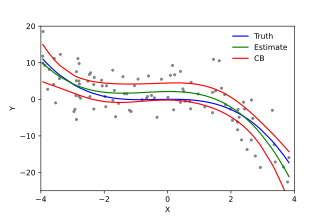
- Ridge regression[15][16][17] and other forms of penalized estimation, such as Lasso regression,[5] deliberately introduce bias into the estimation of β in order to reduce the variability of the estimate. The resulting estimates generally have lower mean squared error than the OLS estimates, particularly when multicollinearity is present or when overfitting is a problem. They are generally used when the goal is to predict the value of the response variable y for values of the predictors x that have not yet been observed. These methods are not as commonly used when the goal is inference, since it is difficult to account for the bias.
- Least absolute deviation (LAD) regression is a robust estimation technique in that it is less sensitive to the presence of outliers than OLS (but is less efficient than OLS when no outliers are present). It is equivalent to maximum likelihood estimation under a Laplace distribution model for ε.[18]
- Adaptive estimation. If we assume that error terms are independent of the regressors, , then the optimal estimator is the 2-step MLE, where the first step is used to non-parametrically estimate the distribution of the error term.[19]

Other estimation techniques[edit]
- Bayesian linear regression applies the framework of Bayesian statistics to linear regression. (See also Bayesian multivariate linear regression.) In particular, the regression coefficients β are assumed to be random variables with a specified prior distribution. The prior distribution can bias the solutions for the regression coefficients, in a way similar to (but more general than) ridge regression or lasso regression. In addition, the Bayesian estimation process produces not a single point estimate for the «best» values of the regression coefficients but an entire posterior distribution, completely describing the uncertainty surrounding the quantity. This can be used to estimate the «best» coefficients using the mean, mode, median, any quantile (see quantile regression), or any other function of the posterior distribution.
- Quantile regression focuses on the conditional quantiles of y given X rather than the conditional mean of y given X. Linear quantile regression models a particular conditional quantile, for example the conditional median, as a linear function βTx of the predictors.
- Mixed models are widely used to analyze linear regression relationships involving dependent data when the dependencies have a known structure. Common applications of mixed models include analysis of data involving repeated measurements, such as longitudinal data, or data obtained from cluster sampling. They are generally fit as parametric models, using maximum likelihood or Bayesian estimation. In the case where the errors are modeled as normal random variables, there is a close connection between mixed models and generalized least squares.[20] Fixed effects estimation is an alternative approach to analyzing this type of data.
- Principal component regression (PCR)[7][8] is used when the number of predictor variables is large, or when strong correlations exist among the predictor variables. This two-stage procedure first reduces the predictor variables using principal component analysis, and then uses the reduced variables in an OLS regression fit. While it often works well in practice, there is no general theoretical reason that the most informative linear function of the predictor variables should lie among the dominant principal components of the multivariate distribution of the predictor variables. The partial least squares regression is the extension of the PCR method which does not suffer from the mentioned deficiency.
- Least-angle regression[6] is an estimation procedure for linear regression models that was developed to handle high-dimensional covariate vectors, potentially with more covariates than observations.
- The Theil–Sen estimator is a simple robust estimation technique that chooses the slope of the fit line to be the median of the slopes of the lines through pairs of sample points. It has similar statistical efficiency properties to simple linear regression but is much less sensitive to outliers.[21]
- Other robust estimation techniques, including the α-trimmed mean approach[citation needed], and L-, M-, S-, and R-estimators have been introduced.[citation needed]
Applications[edit]
Linear regression is widely used in biological, behavioral and social sciences to describe possible relationships between variables. It ranks as one of the most important tools used in these disciplines.
Trend line[edit]
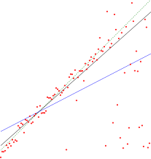
A trend line represents a trend, the long-term movement in time series data after other components have been accounted for. It tells whether a particular data set (say GDP, oil prices or stock prices) have increased or decreased over the period of time. A trend line could simply be drawn by eye through a set of data points, but more properly their position and slope is calculated using statistical techniques like linear regression. Trend lines typically are straight lines, although some variations use higher degree polynomials depending on the degree of curvature desired in the line.
Trend lines are sometimes used in business analytics to show changes in data over time. This has the advantage of being simple. Trend lines are often used to argue that a particular action or event (such as training, or an advertising campaign) caused observed changes at a point in time. This is a simple technique, and does not require a control group, experimental design, or a sophisticated analysis technique. However, it suffers from a lack of scientific validity in cases where other potential changes can affect the data.
Epidemiology[edit]
Early evidence relating tobacco smoking to mortality and morbidity came from observational studies employing regression analysis. In order to reduce spurious correlations when analyzing observational data, researchers usually include several variables in their regression models in addition to the variable of primary interest. For example, in a regression model in which cigarette smoking is the independent variable of primary interest and the dependent variable is lifespan measured in years, researchers might include education and income as additional independent variables, to ensure that any observed effect of smoking on lifespan is not due to those other socio-economic factors. However, it is never possible to include all possible confounding variables in an empirical analysis. For example, a hypothetical gene might increase mortality and also cause people to smoke more. For this reason, randomized controlled trials are often able to generate more compelling evidence of causal relationships than can be obtained using regression analyses of observational data. When controlled experiments are not feasible, variants of regression analysis such as instrumental variables regression may be used to attempt to estimate causal relationships from observational data.
Finance[edit]
The capital asset pricing model uses linear regression as well as the concept of beta for analyzing and quantifying the systematic risk of an investment. This comes directly from the beta coefficient of the linear regression model that relates the return on the investment to the return on all risky assets.
Economics[edit]
Linear regression is the predominant empirical tool in economics. For example, it is used to predict consumption spending,[22] fixed investment spending, inventory investment, purchases of a country’s exports,[23] spending on imports,[23] the demand to hold liquid assets,[24] labor demand,[25] and labor supply.[25]
Environmental science[edit]
|
This section needs expansion. You can help by adding to it. (January 2010) |
Linear regression finds application in a wide range of environmental science applications. In Canada, the Environmental Effects Monitoring Program uses statistical analyses on fish and benthic surveys to measure the effects of pulp mill or metal mine effluent on the aquatic ecosystem.[26]
Machine learning[edit]
Linear regression plays an important role in the subfield of artificial intelligence known as machine learning. The linear regression algorithm is one of the fundamental supervised machine-learning algorithms due to its relative simplicity and well-known properties.[27]
History[edit]
Least squares linear regression, as a means of finding a good rough linear fit to a set of points was performed by Legendre (1805) and Gauss (1809) for the prediction of planetary movement. Quetelet was responsible for making the procedure well-known and for using it extensively in the social sciences.[28]
See also[edit]
- Analysis of variance
- Blinder–Oaxaca decomposition
- Censored regression model
- Cross-sectional regression
- Curve fitting
- Empirical Bayes method
- Errors and residuals
- Lack-of-fit sum of squares
- Line fitting
- Linear classifier
- Linear equation
- Logistic regression
- M-estimator
- Multivariate adaptive regression spline
- Nonlinear regression
- Nonparametric regression
- Normal equations
- Projection pursuit regression
- Response modeling methodology
- Segmented linear regression
- Standard deviation line
- Stepwise regression
- Structural break
- Support vector machine
- Truncated regression model
- Deming regression
References[edit]
Citations[edit]
- ^ David A. Freedman (2009). Statistical Models: Theory and Practice. Cambridge University Press. p. 26.
A simple regression equation has on the right hand side an intercept and an explanatory variable with a slope coefficient. A multiple regression e right hand side, each with its own slope coefficient
- ^ Rencher, Alvin C.; Christensen, William F. (2012), «Chapter 10, Multivariate regression – Section 10.1, Introduction», Methods of Multivariate Analysis, Wiley Series in Probability and Statistics, vol. 709 (3rd ed.), John Wiley & Sons, p. 19, ISBN 9781118391679.
- ^ Hilary L. Seal (1967). «The historical development of the Gauss linear model». Biometrika. 54 (1/2): 1–24. doi:10.1093/biomet/54.1-2.1. JSTOR 2333849.
- ^ Yan, Xin (2009), Linear Regression Analysis: Theory and Computing, World Scientific, pp. 1–2, ISBN 9789812834119,
Regression analysis … is probably one of the oldest topics in mathematical statistics dating back to about two hundred years ago. The earliest form of the linear regression was the least squares method, which was published by Legendre in 1805, and by Gauss in 1809 … Legendre and Gauss both applied the method to the problem of determining, from astronomical observations, the orbits of bodies about the sun.
- ^ a b Tibshirani, Robert (1996). «Regression Shrinkage and Selection via the Lasso». Journal of the Royal Statistical Society, Series B. 58 (1): 267–288. JSTOR 2346178.
- ^ a b Efron, Bradley; Hastie, Trevor; Johnstone, Iain; Tibshirani, Robert (2004). «Least Angle Regression». The Annals of Statistics. 32 (2): 407–451. arXiv:math/0406456. doi:10.1214/009053604000000067. JSTOR 3448465. S2CID 204004121.
- ^ a b Hawkins, Douglas M. (1973). «On the Investigation of Alternative Regressions by Principal Component Analysis». Journal of the Royal Statistical Society, Series C. 22 (3): 275–286. doi:10.2307/2346776. JSTOR 2346776.
- ^ a b Jolliffe, Ian T. (1982). «A Note on the Use of Principal Components in Regression». Journal of the Royal Statistical Society, Series C. 31 (3): 300–303. doi:10.2307/2348005. JSTOR 2348005.
- ^ Berk, Richard A. (2007). «Regression Analysis: A Constructive Critique». Criminal Justice Review. 32 (3): 301–302. doi:10.1177/0734016807304871. S2CID 145389362.
- ^ Tsao, Min (2022). «Group least squares regression for linear models with strongly correlated predictor variables». Annals of the Institute of Statistical Mathematics. arXiv:1804.02499. doi:10.1007/s10463-022-00841-7. S2CID 237396158.
- ^ Hidalgo, Bertha; Goodman, Melody (2012-11-15). «Multivariate or Multivariable Regression?». American Journal of Public Health. 103 (1): 39–40. doi:10.2105/AJPH.2012.300897. ISSN 0090-0036. PMC 3518362. PMID 23153131.
- ^ Brillinger, David R. (1977). «The Identification of a Particular Nonlinear Time Series System». Biometrika. 64 (3): 509–515. doi:10.1093/biomet/64.3.509. JSTOR 2345326.
- ^ Galton, Francis (1886). «Regression Towards Mediocrity in Hereditary Stature». The Journal of the Anthropological Institute of Great Britain and Ireland. 15: 246–263. doi:10.2307/2841583. ISSN 0959-5295. JSTOR 2841583.
- ^ Lange, Kenneth L.; Little, Roderick J. A.; Taylor, Jeremy M. G. (1989). «Robust Statistical Modeling Using the t Distribution» (PDF). Journal of the American Statistical Association. 84 (408): 881–896. doi:10.2307/2290063. JSTOR 2290063.
- ^ Swindel, Benee F. (1981). «Geometry of Ridge Regression Illustrated». The American Statistician. 35 (1): 12–15. doi:10.2307/2683577. JSTOR 2683577.
- ^ Draper, Norman R.; van Nostrand; R. Craig (1979). «Ridge Regression and James-Stein Estimation: Review and Comments». Technometrics. 21 (4): 451–466. doi:10.2307/1268284. JSTOR 1268284.
- ^ Hoerl, Arthur E.; Kennard, Robert W.; Hoerl, Roger W. (1985). «Practical Use of Ridge Regression: A Challenge Met». Journal of the Royal Statistical Society, Series C. 34 (2): 114–120. JSTOR 2347363.
- ^ Narula, Subhash C.; Wellington, John F. (1982). «The Minimum Sum of Absolute Errors Regression: A State of the Art Survey». International Statistical Review. 50 (3): 317–326. doi:10.2307/1402501. JSTOR 1402501.
- ^ Stone, C. J. (1975). «Adaptive maximum likelihood estimators of a location parameter». The Annals of Statistics. 3 (2): 267–284. doi:10.1214/aos/1176343056. JSTOR 2958945.
- ^ Goldstein, H. (1986). «Multilevel Mixed Linear Model Analysis Using Iterative Generalized Least Squares». Biometrika. 73 (1): 43–56. doi:10.1093/biomet/73.1.43. JSTOR 2336270.
- ^ Theil, H. (1950). «A rank-invariant method of linear and polynomial regression analysis. I, II, III». Nederl. Akad. Wetensch., Proc. 53: 386–392, 521–525, 1397–1412. MR 0036489.; Sen, Pranab Kumar (1968). «Estimates of the regression coefficient based on Kendall’s tau». Journal of the American Statistical Association. 63 (324): 1379–1389. doi:10.2307/2285891. JSTOR 2285891. MR 0258201..
- ^ Deaton, Angus (1992). Understanding Consumption. Oxford University Press. ISBN 978-0-19-828824-4.
- ^ a b Krugman, Paul R.; Obstfeld, M.; Melitz, Marc J. (2012). International Economics: Theory and Policy (9th global ed.). Harlow: Pearson. ISBN 9780273754091.
- ^ Laidler, David E. W. (1993). The Demand for Money: Theories, Evidence, and Problems (4th ed.). New York: Harper Collins. ISBN 978-0065010985.
- ^ a b Ehrenberg; Smith (2008). Modern Labor Economics (10th international ed.). London: Addison-Wesley. ISBN 9780321538963.
- ^ EEMP webpage Archived 2011-06-11 at the Wayback Machine
- ^ «Linear Regression (Machine Learning)» (PDF). University of Pittsburgh.
- ^
Stigler, Stephen M. (1986). The History of Statistics: The Measurement of Uncertainty before 1900. Cambridge: Harvard. ISBN 0-674-40340-1.
Sources[edit]
- Cohen, J., Cohen P., West, S.G., & Aiken, L.S. (2003). Applied multiple regression/correlation analysis for the behavioral sciences. (2nd ed.) Hillsdale, NJ: Lawrence Erlbaum Associates
- Charles Darwin. The Variation of Animals and Plants under Domestication. (1868) (Chapter XIII describes what was known about reversion in Galton’s time. Darwin uses the term «reversion».)
- Draper, N.R.; Smith, H. (1998). Applied Regression Analysis (3rd ed.). John Wiley. ISBN 978-0-471-17082-2.
- Francis Galton. «Regression Towards Mediocrity in Hereditary Stature,» Journal of the Anthropological Institute, 15:246-263 (1886). (Facsimile at: [1])
- Robert S. Pindyck and Daniel L. Rubinfeld (1998, 4h ed.). Econometric Models and Economic Forecasts, ch. 1 (Intro, incl. appendices on Σ operators & derivation of parameter est.) & Appendix 4.3 (mult. regression in matrix form).
Further reading[edit]
- Pedhazur, Elazar J (1982). Multiple regression in behavioral research: Explanation and prediction (2nd ed.). New York: Holt, Rinehart and Winston. ISBN 978-0-03-041760-3.
- Mathieu Rouaud, 2013: Probability, Statistics and Estimation Chapter 2: Linear Regression, Linear Regression with Error Bars and Nonlinear Regression.
- National Physical Laboratory (1961). «Chapter 1: Linear Equations and Matrices: Direct Methods». Modern Computing Methods. Notes on Applied Science. Vol. 16 (2nd ed.). Her Majesty’s Stationery Office.
External links[edit]
- Least-Squares Regression, PhET Interactive simulations, University of Colorado at Boulder
- DIY Linear Fit
In statistics, linear regression is a linear approach for modelling the relationship between a scalar response and one or more explanatory variables (also known as dependent and independent variables). The case of one explanatory variable is called simple linear regression; for more than one, the process is called multiple linear regression.[1] This term is distinct from multivariate linear regression, where multiple correlated dependent variables are predicted, rather than a single scalar variable.[2]
In linear regression, the relationships are modeled using linear predictor functions whose unknown model parameters are estimated from the data. Such models are called linear models.[3] Most commonly, the conditional mean of the response given the values of the explanatory variables (or predictors) is assumed to be an affine function of those values; less commonly, the conditional median or some other quantile is used. Like all forms of regression analysis, linear regression focuses on the conditional probability distribution of the response given the values of the predictors, rather than on the joint probability distribution of all of these variables, which is the domain of multivariate analysis.
Linear regression was the first type of regression analysis to be studied rigorously, and to be used extensively in practical applications.[4] This is because models which depend linearly on their unknown parameters are easier to fit than models which are non-linearly related to their parameters and because the statistical properties of the resulting estimators are easier to determine.
Linear regression has many practical uses. Most applications fall into one of the following two broad categories:
- If the goal is error reduction in prediction or forecasting, linear regression can be used to fit a predictive model to an observed data set of values of the response and explanatory variables. After developing such a model, if additional values of the explanatory variables are collected without an accompanying response value, the fitted model can be used to make a prediction of the response.
- If the goal is to explain variation in the response variable that can be attributed to variation in the explanatory variables, linear regression analysis can be applied to quantify the strength of the relationship between the response and the explanatory variables, and in particular to determine whether some explanatory variables may have no linear relationship with the response at all, or to identify which subsets of explanatory variables may contain redundant information about the response.
Linear regression models are often fitted using the least squares approach, but they may also be fitted in other ways, such as by minimizing the «lack of fit» in some other norm (as with least absolute deviations regression), or by minimizing a penalized version of the least squares cost function as in ridge regression (L2-norm penalty) and lasso (L1-norm penalty). Conversely, the least squares approach can be used to fit models that are not linear models. Thus, although the terms «least squares» and «linear model» are closely linked, they are not synonymous.
Formulation[edit]
In linear regression, the observations (red) are assumed to be the result of random deviations (green) from an underlying relationship (blue) between a dependent variable (y) and an independent variable (x).
Given a data set of n statistical units, a linear regression model assumes that the relationship between the dependent variable y and the p-vector of regressors x is linear. This relationship is modeled through a disturbance term or error variable ε — an unobserved random variable that adds «noise» to the linear relationship between the dependent variable and regressors. Thus the model takes the form
where T denotes the transpose, so that xiTβ is the inner product between vectors xi and β.
Often these n equations are stacked together and written in matrix notation as
where
Notation and terminology[edit]
- is a vector of observed values of the variable called the regressand, endogenous variable, response variable, measured variable, criterion variable, or dependent variable. This variable is also sometimes known as the predicted variable, but this should not be confused with predicted values, which are denoted . The decision as to which variable in a data set is modeled as the dependent variable and which are modeled as the independent variables may be based on a presumption that the value of one of the variables is caused by, or directly influenced by the other variables. Alternatively, there may be an operational reason to model one of the variables in terms of the others, in which case there need be no presumption of causality.
- may be seen as a matrix of row-vectors or of n-dimensional column-vectors , which are known as regressors, exogenous variables, explanatory variables, covariates, input variables, predictor variables, or independent variables (not to be confused with the concept of independent random variables). The matrix is sometimes called the design matrix.
- is a -dimensional parameter vector, where is the intercept term (if one is included in the model—otherwise is p-dimensional). Its elements are known as effects or regression coefficients (although the latter term is sometimes reserved for the estimated effects). In simple linear regression, p=1, and the coefficient is known as regression slope. Statistical estimation and inference in linear regression focuses on β. The elements of this parameter vector are interpreted as the partial derivatives of the dependent variable with respect to the various independent variables.
- is a vector of values . This part of the model is called the error term, disturbance term, or sometimes noise (in contrast with the «signal» provided by the rest of the model). This variable captures all other factors which influence the dependent variable y other than the regressors x. The relationship between the error term and the regressors, for example their correlation, is a crucial consideration in formulating a linear regression model, as it will determine the appropriate estimation method.
Fitting a linear model to a given data set usually requires estimating the regression coefficients such that the error term is minimized. For example, it is common to use the sum of squared errors as a measure of for minimization.
Example[edit]
Consider a situation where a small ball is being tossed up in the air and then we measure its heights of ascent hi at various moments in time ti. Physics tells us that, ignoring the drag, the relationship can be modeled as
where β1 determines the initial velocity of the ball, β2 is proportional to the standard gravity, and εi is due to measurement errors. Linear regression can be used to estimate the values of β1 and β2 from the measured data. This model is non-linear in the time variable, but it is linear in the parameters β1 and β2; if we take regressors xi = (xi1, xi2) = (ti, ti2), the model takes on the standard form
Assumptions[edit]
Standard linear regression models with standard estimation techniques make a number of assumptions about the predictor variables, the response variables and their relationship. Numerous extensions have been developed that allow each of these assumptions to be relaxed (i.e. reduced to a weaker form), and in some cases eliminated entirely. Generally these extensions make the estimation procedure more complex and time-consuming, and may also require more data in order to produce an equally precise model.
Example of a cubic polynomial regression, which is a type of linear regression. Although polynomial regression fits a nonlinear model to the data, as a statistical estimation problem it is linear, in the sense that the regression function E(y | x) is linear in the unknown parameters that are estimated from the data. For this reason, polynomial regression is considered to be a special case of multiple linear regression.
The following are the major assumptions made by standard linear regression models with standard estimation techniques (e.g. ordinary least squares):
- Weak exogeneity. This essentially means that the predictor variables x can be treated as fixed values, rather than random variables. This means, for example, that the predictor variables are assumed to be error-free—that is, not contaminated with measurement errors. Although this assumption is not realistic in many settings, dropping it leads to significantly more difficult errors-in-variables models.
- Linearity. This means that the mean of the response variable is a linear combination of the parameters (regression coefficients) and the predictor variables. Note that this assumption is much less restrictive than it may at first seem. Because the predictor variables are treated as fixed values (see above), linearity is really only a restriction on the parameters. The predictor variables themselves can be arbitrarily transformed, and in fact multiple copies of the same underlying predictor variable can be added, each one transformed differently. This technique is used, for example, in polynomial regression, which uses linear regression to fit the response variable as an arbitrary polynomial function (up to a given degree) of a predictor variable. With this much flexibility, models such as polynomial regression often have «too much power», in that they tend to overfit the data. As a result, some kind of regularization must typically be used to prevent unreasonable solutions coming out of the estimation process. Common examples are ridge regression and lasso regression. Bayesian linear regression can also be used, which by its nature is more or less immune to the problem of overfitting. (In fact, ridge regression and lasso regression can both be viewed as special cases of Bayesian linear regression, with particular types of prior distributions placed on the regression coefficients.)
- Constant variance (a.k.a. homoscedasticity). This means that the variance of the errors does not depend on the values of the predictor variables. Thus the variability of the responses for given fixed values of the predictors is the same regardless of how large or small the responses are. This is often not the case, as a variable whose mean is large will typically have a greater variance than one whose mean is small. For example, a person whose income is predicted to be $100,000 may easily have an actual income of $80,000 or $120,000—i.e., a standard deviation of around $20,000—while another person with a predicted income of $10,000 is unlikely to have the same $20,000 standard deviation, since that would imply their actual income could vary anywhere between −$10,000 and $30,000. (In fact, as this shows, in many cases—often the same cases where the assumption of normally distributed errors fails—the variance or standard deviation should be predicted to be proportional to the mean, rather than constant.) The absence of homoscedasticity is called heteroscedasticity. In order to check this assumption, a plot of residuals versus predicted values (or the values of each individual predictor) can be examined for a «fanning effect» (i.e., increasing or decreasing vertical spread as one moves left to right on the plot). A plot of the absolute or squared residuals versus the predicted values (or each predictor) can also be examined for a trend or curvature. Formal tests can also be used; see Heteroscedasticity. The presence of heteroscedasticity will result in an overall «average» estimate of variance being used instead of one that takes into account the true variance structure. This leads to less precise (but in the case of ordinary least squares, not biased) parameter estimates and biased standard errors, resulting in misleading tests and interval estimates. The mean squared error for the model will also be wrong. Various estimation techniques including weighted least squares and the use of heteroscedasticity-consistent standard errors can handle heteroscedasticity in a quite general way. Bayesian linear regression techniques can also be used when the variance is assumed to be a function of the mean. It is also possible in some cases to fix the problem by applying a transformation to the response variable (e.g., fitting the logarithm of the response variable using a linear regression model, which implies that the response variable itself has a log-normal distribution rather than a normal distribution).
To check for violations of the assumptions of linearity, constant variance, and independence of errors within a linear regression model, the residuals are typically plotted against the predicted values (or each of the individual predictors). An apparently random scatter of points about the horizontal midline at 0 is ideal, but cannot rule out certain kinds of violations such as autocorrelation in the errors or their correlation with one or more covariates.
- Independence of errors. This assumes that the errors of the response variables are uncorrelated with each other. (Actual statistical independence is a stronger condition than mere lack of correlation and is often not needed, although it can be exploited if it is known to hold.) Some methods such as generalized least squares are capable of handling correlated errors, although they typically require significantly more data unless some sort of regularization is used to bias the model towards assuming uncorrelated errors. Bayesian linear regression is a general way of handling this issue.
- Lack of perfect multicollinearity in the predictors. For standard least squares estimation methods, the design matrix X must have full column rank p; otherwise perfect multicollinearity exists in the predictor variables, meaning a linear relationship exists between two or more predictor variables. This can be caused by accidentally duplicating a variable in the data, using a linear transformation of a variable along with the original (e.g., the same temperature measurements expressed in Fahrenheit and Celsius), or including a linear combination of multiple variables in the model, such as their mean. It can also happen if there is too little data available compared to the number of parameters to be estimated (e.g., fewer data points than regression coefficients). Near violations of this assumption, where predictors are highly but not perfectly correlated, can reduce the precision of parameter estimates (see Variance inflation factor). In the case of perfect multicollinearity, the parameter vector β will be non-identifiable—it has no unique solution. In such a case, only some of the parameters can be identified (i.e., their values can only be estimated within some linear subspace of the full parameter space Rp). See partial least squares regression. Methods for fitting linear models with multicollinearity have been developed,[5][6][7][8] some of which require additional assumptions such as «effect sparsity»—that a large fraction of the effects are exactly zero. Note that the more computationally expensive iterated algorithms for parameter estimation, such as those used in generalized linear models, do not suffer from this problem.
Beyond these assumptions, several other statistical properties of the data strongly influence the performance of different estimation methods:
- The statistical relationship between the error terms and the regressors plays an important role in determining whether an estimation procedure has desirable sampling properties such as being unbiased and consistent.
- The arrangement, or probability distribution of the predictor variables x has a major influence on the precision of estimates of β. Sampling and design of experiments are highly developed subfields of statistics that provide guidance for collecting data in such a way to achieve a precise estimate of β.
Interpretation[edit]
The data sets in the Anscombe’s quartet are designed to have approximately the same linear regression line (as well as nearly identical means, standard deviations, and correlations) but are graphically very different. This illustrates the pitfalls of relying solely on a fitted model to understand the relationship between variables.
A fitted linear regression model can be used to identify the relationship between a single predictor variable xj and the response variable y when all the other predictor variables in the model are «held fixed». Specifically, the interpretation of βj is the expected change in y for a one-unit change in xj when the other covariates are held fixed—that is, the expected value of the partial derivative of y with respect to xj. This is sometimes called the unique effect of xj on y. In contrast, the marginal effect of xj on y can be assessed using a correlation coefficient or simple linear regression model relating only xj to y; this effect is the total derivative of y with respect to xj.
Care must be taken when interpreting regression results, as some of the regressors may not allow for marginal changes (such as dummy variables, or the intercept term), while others cannot be held fixed (recall the example from the introduction: it would be impossible to «hold ti fixed» and at the same time change the value of ti2).
It is possible that the unique effect can be nearly zero even when the marginal effect is large. This may imply that some other covariate captures all the information in xj, so that once that variable is in the model, there is no contribution of xj to the variation in y. Conversely, the unique effect of xj can be large while its marginal effect is nearly zero. This would happen if the other covariates explained a great deal of the variation of y, but they mainly explain variation in a way that is complementary to what is captured by xj. In this case, including the other variables in the model reduces the part of the variability of y that is unrelated to xj, thereby strengthening the apparent relationship with xj.
The meaning of the expression «held fixed» may depend on how the values of the predictor variables arise. If the experimenter directly sets the values of the predictor variables according to a study design, the comparisons of interest may literally correspond to comparisons among units whose predictor variables have been «held fixed» by the experimenter. Alternatively, the expression «held fixed» can refer to a selection that takes place in the context of data analysis. In this case, we «hold a variable fixed» by restricting our attention to the subsets of the data that happen to have a common value for the given predictor variable. This is the only interpretation of «held fixed» that can be used in an observational study.
The notion of a «unique effect» is appealing when studying a complex system where multiple interrelated components influence the response variable. In some cases, it can literally be interpreted as the causal effect of an intervention that is linked to the value of a predictor variable. However, it has been argued that in many cases multiple regression analysis fails to clarify the relationships between the predictor variables and the response variable when the predictors are correlated with each other and are not assigned following a study design.[9]
Group effects[edit]
In a multiple linear regression model
parameter of predictor variable represents the individual effect of . It has an interpretation as the expected change in the response variable when increases by one unit with other predictor variables held constant. When is strongly correlated with other predictor variables, it is improbable that can increase by one unit with other variables held constant. In this case, the interpretation of becomes problematic as it is based on an improbable condition, and the effect of cannot be evaluated in isolation.
For a group of predictor variables, say, , a group effect is defined as a linear combination of their parameters
where is a weight vector satisfying . Because of the constraint on , is also referred to as a normalized group effect. A group effect has an interpretation as the expected change in when variables in the group change by the amount , respectively, at the same time with variables not in the group held constant. It generalizes the individual effect of a variable to a group of variables in that () if , then the group effect reduces to an individual effect, and () if and for , then the group effect also reduces to an individual effect.
A group effect is said to be meaningful if the underlying simultaneous changes of the variables is probable.
Group effects provide a means to study the collective impact of strongly correlated predictor variables in linear regression models. Individual effects of such variables are not well-defined as their parameters do not have good interpretations. Furthermore, when the sample size is not large, none of their parameters can be accurately estimated by the least squares regression due to the multicollinearity problem. Nevertheless, there are meaningful group effects that have good interpretations and can be accurately estimated by the least squares regression. A simple way to identify these meaningful group effects is to use an all positive correlations (APC) arrangement of the strongly correlated variables under which pairwise correlations among these variables are all positive, and standardize all predictor variables in the model so that they all have mean zero and length one. To illustrate this, suppose that is a group of strongly correlated variables in an APC arrangement and that they are not strongly correlated with predictor variables outside the group. Let be the centred and be the standardized . Then, the standardized linear regression model is
Parameters in the original model, including , are simple functions of in the standardized model. The standardization of variables does not change their correlations, so is a group of strongly correlated variables in an APC arrangement and they are not strongly correlated with other predictor variables in the standardized model. A group effect of is
and its minimum-variance unbiased linear estimator is
where is the least squares estimator of . In particular, the average group effect of the standardized variables is
which has an interpretation as the expected change in when all in the strongly correlated group increase by th of a unit at the same time with variables outside the group held constant. With strong positive correlations and in standardized units, variables in the group are approximately equal, so they are likely to increase at the same time and in similar amount. Thus, the average group effect is a meaningful effect. It can be accurately estimated by its minimum-variance unbiased linear estimator , even when individually none of the can be accurately estimated by .
Not all group effects are meaningful or can be accurately estimated. For example, is a special group effect with weights and for , but it cannot be accurately estimated by . It is also not a meaningful effect. In general, for a group of strongly correlated predictor variables in an APC arrangement in the standardized model, group effects whose weight vectors are at or near the centre of the simplex () are meaningful and can be accurately estimated by their minimum-variance unbiased linear estimators. Effects with weight vectors far away from the centre are not meaningful as such weight vectors represent simultaneous changes of the variables that violate the strong positive correlations of the standardized variables in an APC arrangement. As such, they are not probable. These effects also cannot be accurately estimated.
Applications of the group effects include (1) estimation and inference for meaningful group effects on the response variable, (2) testing for «group significance» of the variables via testing versus , and (3) characterizing the region of the predictor variable space over which predictions by the least squares estimated model are accurate.
A group effect of the original variables can be expressed as a constant times a group effect of the standardized variables . The former is meaningful when the latter is. Thus meaningful group effects of the original variables can be found through meaningful group effects of the standardized variables.[10]
Extensions[edit]
Numerous extensions of linear regression have been developed, which allow some or all of the assumptions underlying the basic model to be relaxed.
Simple and multiple linear regression[edit]
The very simplest case of a single scalar predictor variable x and a single scalar response variable y is known as simple linear regression. The extension to multiple and/or vector-valued predictor variables (denoted with a capital X) is known as multiple linear regression, also known as multivariable linear regression (not to be confused with multivariate linear regression[11]).
Multiple linear regression is a generalization of simple linear regression to the case of more than one independent variable, and a special case of general linear models, restricted to one dependent variable. The basic model for multiple linear regression is
for each observation i = 1, … , n.
In the formula above we consider n observations of one dependent variable and p independent variables. Thus, Yi is the ith observation of the dependent variable, Xij is ith observation of the jth independent variable, j = 1, 2, …, p. The values βj represent parameters to be estimated, and εi is the ith independent identically distributed normal error.
In the more general multivariate linear regression, there is one equation of the above form for each of m > 1 dependent variables that share the same set of explanatory variables and hence are estimated simultaneously with each other:
for all observations indexed as i = 1, … , n and for all dependent variables indexed as j = 1, … , m.
Nearly all real-world regression models involve multiple predictors, and basic descriptions of linear regression are often phrased in terms of the multiple regression model. Note, however, that in these cases the response variable y is still a scalar. Another term, multivariate linear regression, refers to cases where y is a vector, i.e., the same as general linear regression.
General linear models[edit]
The general linear model considers the situation when the response variable is not a scalar (for each observation) but a vector, yi. Conditional linearity of is still assumed, with a matrix B replacing the vector β of the classical linear regression model. Multivariate analogues of ordinary least squares (OLS) and generalized least squares (GLS) have been developed. «General linear models» are also called «multivariate linear models». These are not the same as multivariable linear models (also called «multiple linear models»).
Heteroscedastic models[edit]
Various models have been created that allow for heteroscedasticity, i.e. the errors for different response variables may have different variances. For example, weighted least squares is a method for estimating linear regression models when the response variables may have different error variances, possibly with correlated errors. (See also Weighted linear least squares, and Generalized least squares.) Heteroscedasticity-consistent standard errors is an improved method for use with uncorrelated but potentially heteroscedastic errors.
Generalized linear models[edit]
Generalized linear models (GLMs) are a framework for modeling response variables that are bounded or discrete. This is used, for example:
- when modeling positive quantities (e.g. prices or populations) that vary over a large scale—which are better described using a skewed distribution such as the log-normal distribution or Poisson distribution (although GLMs are not used for log-normal data, instead the response variable is simply transformed using the logarithm function);
- when modeling categorical data, such as the choice of a given candidate in an election (which is better described using a Bernoulli distribution/binomial distribution for binary choices, or a categorical distribution/multinomial distribution for multi-way choices), where there are a fixed number of choices that cannot be meaningfully ordered;
- when modeling ordinal data, e.g. ratings on a scale from 0 to 5, where the different outcomes can be ordered but where the quantity itself may not have any absolute meaning (e.g. a rating of 4 may not be «twice as good» in any objective sense as a rating of 2, but simply indicates that it is better than 2 or 3 but not as good as 5).
Generalized linear models allow for an arbitrary link function, g, that relates the mean of the response variable(s) to the predictors: . The link function is often related to the distribution of the response, and in particular it typically has the effect of transforming between the range of the linear predictor and the range of the response variable.
Some common examples of GLMs are:
- Poisson regression for count data.
- Logistic regression and probit regression for binary data.
- Multinomial logistic regression and multinomial probit regression for categorical data.
- Ordered logit and ordered probit regression for ordinal data.
Single index models[clarification needed] allow some degree of nonlinearity in the relationship between x and y, while preserving the central role of the linear predictor β′x as in the classical linear regression model. Under certain conditions, simply applying OLS to data from a single-index model will consistently estimate β up to a proportionality constant.[12]
Hierarchical linear models[edit]
Hierarchical linear models (or multilevel regression) organizes the data into a hierarchy of regressions, for example where A is regressed on B, and B is regressed on C. It is often used where the variables of interest have a natural hierarchical structure such as in educational statistics, where students are nested in classrooms, classrooms are nested in schools, and schools are nested in some administrative grouping, such as a school district. The response variable might be a measure of student achievement such as a test score, and different covariates would be collected at the classroom, school, and school district levels.
Errors-in-variables[edit]
Errors-in-variables models (or «measurement error models») extend the traditional linear regression model to allow the predictor variables X to be observed with error. This error causes standard estimators of β to become biased. Generally, the form of bias is an attenuation, meaning that the effects are biased toward zero.
Others[edit]
- In Dempster–Shafer theory, or a linear belief function in particular, a linear regression model may be represented as a partially swept matrix, which can be combined with similar matrices representing observations and other assumed normal distributions and state equations. The combination of swept or unswept matrices provides an alternative method for estimating linear regression models.
Estimation methods[edit]
A large number of procedures have been developed for parameter estimation and inference in linear regression. These methods differ in computational simplicity of algorithms, presence of a closed-form solution, robustness with respect to heavy-tailed distributions, and theoretical assumptions needed to validate desirable statistical properties such as consistency and asymptotic efficiency.
Some of the more common estimation techniques for linear regression are summarized below.
Least-squares estimation and related techniques[edit]
Francis Galton’s 1886[13] illustration of the correlation between the heights of adults and their parents. The observation that adult children’s heights tended to deviate less from the mean height than their parents suggested the concept of «regression toward the mean», giving regression its name. The «locus of horizontal tangential points» passing through the leftmost and rightmost points on the ellipse (which is a level curve of the bivariate normal distribution estimated from the data) is the OLS estimate of the regression of parents’ heights on children’s heights, while the «locus of vertical tangential points» is the OLS estimate of the regression of children’s heights on parent’s heights. The major axis of the ellipse is the TLS estimate.
Assuming that the independent variable is and the model’s parameters are , then the model’s prediction would be
- .
If is extended to then would become a dot product of the parameter and the independent variable, i.e.
- .
In the least-squares setting, the optimum parameter is defined as such that minimizes the sum of mean squared loss:
Now putting the independent and dependent variables in matrices and respectively, the loss function can be rewritten as:
As the loss is convex the optimum solution lies at gradient zero. The gradient of the loss function is (using Denominator layout convention):
Setting the gradient to zero produces the optimum parameter:
Note: To prove that the obtained is indeed the local minimum, one needs to differentiate once more to obtain the Hessian matrix and show that it is positive definite. This is provided by the Gauss–Markov theorem.
Linear least squares methods include mainly:
- Ordinary least squares
- Weighted least squares
- Generalized least squares
Maximum-likelihood estimation and related techniques[edit]
- Maximum likelihood estimation can be performed when the distribution of the error terms is known to belong to a certain parametric family ƒθ of probability distributions.[14] When fθ is a normal distribution with zero mean and variance θ, the resulting estimate is identical to the OLS estimate. GLS estimates are maximum likelihood estimates when ε follows a multivariate normal distribution with a known covariance matrix.
- Ridge regression[15][16][17] and other forms of penalized estimation, such as Lasso regression,[5] deliberately introduce bias into the estimation of β in order to reduce the variability of the estimate. The resulting estimates generally have lower mean squared error than the OLS estimates, particularly when multicollinearity is present or when overfitting is a problem. They are generally used when the goal is to predict the value of the response variable y for values of the predictors x that have not yet been observed. These methods are not as commonly used when the goal is inference, since it is difficult to account for the bias.
- Least absolute deviation (LAD) regression is a robust estimation technique in that it is less sensitive to the presence of outliers than OLS (but is less efficient than OLS when no outliers are present). It is equivalent to maximum likelihood estimation under a Laplace distribution model for ε.[18]
- Adaptive estimation. If we assume that error terms are independent of the regressors, , then the optimal estimator is the 2-step MLE, where the first step is used to non-parametrically estimate the distribution of the error term.[19]
Other estimation techniques[edit]
- Bayesian linear regression applies the framework of Bayesian statistics to linear regression. (See also Bayesian multivariate linear regression.) In particular, the regression coefficients β are assumed to be random variables with a specified prior distribution. The prior distribution can bias the solutions for the regression coefficients, in a way similar to (but more general than) ridge regression or lasso regression. In addition, the Bayesian estimation process produces not a single point estimate for the «best» values of the regression coefficients but an entire posterior distribution, completely describing the uncertainty surrounding the quantity. This can be used to estimate the «best» coefficients using the mean, mode, median, any quantile (see quantile regression), or any other function of the posterior distribution.
- Quantile regression focuses on the conditional quantiles of y given X rather than the conditional mean of y given X. Linear quantile regression models a particular conditional quantile, for example the conditional median, as a linear function βTx of the predictors.
- Mixed models are widely used to analyze linear regression relationships involving dependent data when the dependencies have a known structure. Common applications of mixed models include analysis of data involving repeated measurements, such as longitudinal data, or data obtained from cluster sampling. They are generally fit as parametric models, using maximum likelihood or Bayesian estimation. In the case where the errors are modeled as normal random variables, there is a close connection between mixed models and generalized least squares.[20] Fixed effects estimation is an alternative approach to analyzing this type of data.
- Principal component regression (PCR)[7][8] is used when the number of predictor variables is large, or when strong correlations exist among the predictor variables. This two-stage procedure first reduces the predictor variables using principal component analysis, and then uses the reduced variables in an OLS regression fit. While it often works well in practice, there is no general theoretical reason that the most informative linear function of the predictor variables should lie among the dominant principal components of the multivariate distribution of the predictor variables. The partial least squares regression is the extension of the PCR method which does not suffer from the mentioned deficiency.
- Least-angle regression[6] is an estimation procedure for linear regression models that was developed to handle high-dimensional covariate vectors, potentially with more covariates than observations.
- The Theil–Sen estimator is a simple robust estimation technique that chooses the slope of the fit line to be the median of the slopes of the lines through pairs of sample points. It has similar statistical efficiency properties to simple linear regression but is much less sensitive to outliers.[21]
- Other robust estimation techniques, including the α-trimmed mean approach[citation needed], and L-, M-, S-, and R-estimators have been introduced.[citation needed]
Applications[edit]
Linear regression is widely used in biological, behavioral and social sciences to describe possible relationships between variables. It ranks as one of the most important tools used in these disciplines.
Trend line[edit]
A trend line represents a trend, the long-term movement in time series data after other components have been accounted for. It tells whether a particular data set (say GDP, oil prices or stock prices) have increased or decreased over the period of time. A trend line could simply be drawn by eye through a set of data points, but more properly their position and slope is calculated using statistical techniques like linear regression. Trend lines typically are straight lines, although some variations use higher degree polynomials depending on the degree of curvature desired in the line.
Trend lines are sometimes used in business analytics to show changes in data over time. This has the advantage of being simple. Trend lines are often used to argue that a particular action or event (such as training, or an advertising campaign) caused observed changes at a point in time. This is a simple technique, and does not require a control group, experimental design, or a sophisticated analysis technique. However, it suffers from a lack of scientific validity in cases where other potential changes can affect the data.
Epidemiology[edit]
Early evidence relating tobacco smoking to mortality and morbidity came from observational studies employing regression analysis. In order to reduce spurious correlations when analyzing observational data, researchers usually include several variables in their regression models in addition to the variable of primary interest. For example, in a regression model in which cigarette smoking is the independent variable of primary interest and the dependent variable is lifespan measured in years, researchers might include education and income as additional independent variables, to ensure that any observed effect of smoking on lifespan is not due to those other socio-economic factors. However, it is never possible to include all possible confounding variables in an empirical analysis. For example, a hypothetical gene might increase mortality and also cause people to smoke more. For this reason, randomized controlled trials are often able to generate more compelling evidence of causal relationships than can be obtained using regression analyses of observational data. When controlled experiments are not feasible, variants of regression analysis such as instrumental variables regression may be used to attempt to estimate causal relationships from observational data.
Finance[edit]
The capital asset pricing model uses linear regression as well as the concept of beta for analyzing and quantifying the systematic risk of an investment. This comes directly from the beta coefficient of the linear regression model that relates the return on the investment to the return on all risky assets.
Economics[edit]
Linear regression is the predominant empirical tool in economics. For example, it is used to predict consumption spending,[22] fixed investment spending, inventory investment, purchases of a country’s exports,[23] spending on imports,[23] the demand to hold liquid assets,[24] labor demand,[25] and labor supply.[25]
Environmental science[edit]
|
This section needs expansion. You can help by adding to it. (January 2010) |
Linear regression finds application in a wide range of environmental science applications. In Canada, the Environmental Effects Monitoring Program uses statistical analyses on fish and benthic surveys to measure the effects of pulp mill or metal mine effluent on the aquatic ecosystem.[26]
Machine learning[edit]
Linear regression plays an important role in the subfield of artificial intelligence known as machine learning. The linear regression algorithm is one of the fundamental supervised machine-learning algorithms due to its relative simplicity and well-known properties.[27]
History[edit]
Least squares linear regression, as a means of finding a good rough linear fit to a set of points was performed by Legendre (1805) and Gauss (1809) for the prediction of planetary movement. Quetelet was responsible for making the procedure well-known and for using it extensively in the social sciences.[28]
See also[edit]
- Analysis of variance
- Blinder–Oaxaca decomposition
- Censored regression model
- Cross-sectional regression
- Curve fitting
- Empirical Bayes method
- Errors and residuals
- Lack-of-fit sum of squares
- Line fitting
- Linear classifier
- Linear equation
- Logistic regression
- M-estimator
- Multivariate adaptive regression spline
- Nonlinear regression
- Nonparametric regression
- Normal equations
- Projection pursuit regression
- Response modeling methodology
- Segmented linear regression
- Standard deviation line
- Stepwise regression
- Structural break
- Support vector machine
- Truncated regression model
- Deming regression
References[edit]
Citations[edit]
- ^ David A. Freedman (2009). Statistical Models: Theory and Practice. Cambridge University Press. p. 26.
A simple regression equation has on the right hand side an intercept and an explanatory variable with a slope coefficient. A multiple regression e right hand side, each with its own slope coefficient
- ^ Rencher, Alvin C.; Christensen, William F. (2012), «Chapter 10, Multivariate regression – Section 10.1, Introduction», Methods of Multivariate Analysis, Wiley Series in Probability and Statistics, vol. 709 (3rd ed.), John Wiley & Sons, p. 19, ISBN 9781118391679.
- ^ Hilary L. Seal (1967). «The historical development of the Gauss linear model». Biometrika. 54 (1/2): 1–24. doi:10.1093/biomet/54.1-2.1. JSTOR 2333849.
- ^ Yan, Xin (2009), Linear Regression Analysis: Theory and Computing, World Scientific, pp. 1–2, ISBN 9789812834119,
Regression analysis … is probably one of the oldest topics in mathematical statistics dating back to about two hundred years ago. The earliest form of the linear regression was the least squares method, which was published by Legendre in 1805, and by Gauss in 1809 … Legendre and Gauss both applied the method to the problem of determining, from astronomical observations, the orbits of bodies about the sun.
- ^ a b Tibshirani, Robert (1996). «Regression Shrinkage and Selection via the Lasso». Journal of the Royal Statistical Society, Series B. 58 (1): 267–288. JSTOR 2346178.
- ^ a b Efron, Bradley; Hastie, Trevor; Johnstone, Iain; Tibshirani, Robert (2004). «Least Angle Regression». The Annals of Statistics. 32 (2): 407–451. arXiv:math/0406456. doi:10.1214/009053604000000067. JSTOR 3448465. S2CID 204004121.
- ^ a b Hawkins, Douglas M. (1973). «On the Investigation of Alternative Regressions by Principal Component Analysis». Journal of the Royal Statistical Society, Series C. 22 (3): 275–286. doi:10.2307/2346776. JSTOR 2346776.
- ^ a b Jolliffe, Ian T. (1982). «A Note on the Use of Principal Components in Regression». Journal of the Royal Statistical Society, Series C. 31 (3): 300–303. doi:10.2307/2348005. JSTOR 2348005.
- ^ Berk, Richard A. (2007). «Regression Analysis: A Constructive Critique». Criminal Justice Review. 32 (3): 301–302. doi:10.1177/0734016807304871. S2CID 145389362.
- ^ Tsao, Min (2022). «Group least squares regression for linear models with strongly correlated predictor variables». Annals of the Institute of Statistical Mathematics. arXiv:1804.02499. doi:10.1007/s10463-022-00841-7. S2CID 237396158.
- ^ Hidalgo, Bertha; Goodman, Melody (2012-11-15). «Multivariate or Multivariable Regression?». American Journal of Public Health. 103 (1): 39–40. doi:10.2105/AJPH.2012.300897. ISSN 0090-0036. PMC 3518362. PMID 23153131.
- ^ Brillinger, David R. (1977). «The Identification of a Particular Nonlinear Time Series System». Biometrika. 64 (3): 509–515. doi:10.1093/biomet/64.3.509. JSTOR 2345326.
- ^ Galton, Francis (1886). «Regression Towards Mediocrity in Hereditary Stature». The Journal of the Anthropological Institute of Great Britain and Ireland. 15: 246–263. doi:10.2307/2841583. ISSN 0959-5295. JSTOR 2841583.
- ^ Lange, Kenneth L.; Little, Roderick J. A.; Taylor, Jeremy M. G. (1989). «Robust Statistical Modeling Using the t Distribution» (PDF). Journal of the American Statistical Association. 84 (408): 881–896. doi:10.2307/2290063. JSTOR 2290063.
- ^ Swindel, Benee F. (1981). «Geometry of Ridge Regression Illustrated». The American Statistician. 35 (1): 12–15. doi:10.2307/2683577. JSTOR 2683577.
- ^ Draper, Norman R.; van Nostrand; R. Craig (1979). «Ridge Regression and James-Stein Estimation: Review and Comments». Technometrics. 21 (4): 451–466. doi:10.2307/1268284. JSTOR 1268284.
- ^ Hoerl, Arthur E.; Kennard, Robert W.; Hoerl, Roger W. (1985). «Practical Use of Ridge Regression: A Challenge Met». Journal of the Royal Statistical Society, Series C. 34 (2): 114–120. JSTOR 2347363.
- ^ Narula, Subhash C.; Wellington, John F. (1982). «The Minimum Sum of Absolute Errors Regression: A State of the Art Survey». International Statistical Review. 50 (3): 317–326. doi:10.2307/1402501. JSTOR 1402501.
- ^ Stone, C. J. (1975). «Adaptive maximum likelihood estimators of a location parameter». The Annals of Statistics. 3 (2): 267–284. doi:10.1214/aos/1176343056. JSTOR 2958945.
- ^ Goldstein, H. (1986). «Multilevel Mixed Linear Model Analysis Using Iterative Generalized Least Squares». Biometrika. 73 (1): 43–56. doi:10.1093/biomet/73.1.43. JSTOR 2336270.
- ^ Theil, H. (1950). «A rank-invariant method of linear and polynomial regression analysis. I, II, III». Nederl. Akad. Wetensch., Proc. 53: 386–392, 521–525, 1397–1412. MR 0036489.; Sen, Pranab Kumar (1968). «Estimates of the regression coefficient based on Kendall’s tau». Journal of the American Statistical Association. 63 (324): 1379–1389. doi:10.2307/2285891. JSTOR 2285891. MR 0258201..
- ^ Deaton, Angus (1992). Understanding Consumption. Oxford University Press. ISBN 978-0-19-828824-4.
- ^ a b Krugman, Paul R.; Obstfeld, M.; Melitz, Marc J. (2012). International Economics: Theory and Policy (9th global ed.). Harlow: Pearson. ISBN 9780273754091.
- ^ Laidler, David E. W. (1993). The Demand for Money: Theories, Evidence, and Problems (4th ed.). New York: Harper Collins. ISBN 978-0065010985.
- ^ a b Ehrenberg; Smith (2008). Modern Labor Economics (10th international ed.). London: Addison-Wesley. ISBN 9780321538963.
- ^ EEMP webpage Archived 2011-06-11 at the Wayback Machine
- ^ «Linear Regression (Machine Learning)» (PDF). University of Pittsburgh.
- ^
Stigler, Stephen M. (1986). The History of Statistics: The Measurement of Uncertainty before 1900. Cambridge: Harvard. ISBN 0-674-40340-1.
Sources[edit]
- Cohen, J., Cohen P., West, S.G., & Aiken, L.S. (2003). Applied multiple regression/correlation analysis for the behavioral sciences. (2nd ed.) Hillsdale, NJ: Lawrence Erlbaum Associates
- Charles Darwin. The Variation of Animals and Plants under Domestication. (1868) (Chapter XIII describes what was known about reversion in Galton’s time. Darwin uses the term «reversion».)
- Draper, N.R.; Smith, H. (1998). Applied Regression Analysis (3rd ed.). John Wiley. ISBN 978-0-471-17082-2.
- Francis Galton. «Regression Towards Mediocrity in Hereditary Stature,» Journal of the Anthropological Institute, 15:246-263 (1886). (Facsimile at: [1])
- Robert S. Pindyck and Daniel L. Rubinfeld (1998, 4h ed.). Econometric Models and Economic Forecasts, ch. 1 (Intro, incl. appendices on Σ operators & derivation of parameter est.) & Appendix 4.3 (mult. regression in matrix form).
Further reading[edit]
- Pedhazur, Elazar J (1982). Multiple regression in behavioral research: Explanation and prediction (2nd ed.). New York: Holt, Rinehart and Winston. ISBN 978-0-03-041760-3.
- Mathieu Rouaud, 2013: Probability, Statistics and Estimation Chapter 2: Linear Regression, Linear Regression with Error Bars and Nonlinear Regression.
- National Physical Laboratory (1961). «Chapter 1: Linear Equations and Matrices: Direct Methods». Modern Computing Methods. Notes on Applied Science. Vol. 16 (2nd ed.). Her Majesty’s Stationery Office.
External links[edit]
- Least-Squares Regression, PhET Interactive simulations, University of Colorado at Boulder
- DIY Linear Fit
Регрессия как задача машинного обучения
38 мин на чтение
(55.116 символов)
Постановка задачи регрессии

Источник: Analytics Vidhya.
Задача регрессии — это одна из основных задач машинного обучения. И хотя, большинство задач на практике относятся к другому типу — классификации, мы начнем знакомство с машинным обучением именно с регрессии. Регрессионные модели были известны задолго до появления машинного обучения как отрасли и активно применяются в статистике, эконометрике, математическом моделировании. Машинное обучение предлагает новый взгляд на уже известные модели. И этот новый взгляд позволит строить более сложные и мощные модели, чем классические математические дисциплины.
Задача регрессии относится к категории задач обучения с учителем. Это значит, что набор данных, который используется для обучения, должен иметь определенную структуру. Обычно, наборы данных для машинного обучения представляют собой таблицу, в которой по строкам перечислены разные объекты наблюдений или измерений. В столбцах — различные характеристики, или атрибуты, объектов. А на пересечении строк и столбцов — значение данной характеристики у данного объекта. Обычно один атрибут (или переменная) имеет особый характер — именно ее значение мы и хотим научиться предсказывать с помощью модели машинного обучения. Эта характеристика объекта называется целевая переменная. И если эта целевая переменная выражена числом (а точнее, некоторой непрерывной величиной) — то мы говорим о задаче регрессии.
Задачи регрессии на практике встречаются довольно часто. Например, предсказание цены объекта недвижимости — классическая регрессионная задача. В таких проблемах атрибутами выступают разные характеристики квартир или домов — площадь, этажность, расположение, расстояние до центра города, количество комнат, год постройки. В разных наборах данных собрана разная информация И, соответственно, модели тоже должны быть разные. Другой пример — предсказание цены акций или других финансовых активов. Или предсказание температуры завтрашним днем.
Во всех таких задачах нам нужно иметь данные, которые позволят осуществить такое предсказание. Да, “предсказание” — это условный термин, не всегда мы говорим о будущих событиях. Регрессионные модели используют информацию об объектах в обучающем наборе данных, чтобы сделать вывод о возможном значении целевой переменной. И для этого нужно, чтобы ее значение имело какую-то зависимость от имеющихся у нас атрибутов. Если построить модель предсказания цены акции, но на вход подать информацию о футбольных матчах — ничего не получится. Мы предполагаем, что в наборе данных собраны именно те атрибуты объектов, которые имеют влияние на на значение целевой переменной. И чем больше это предположение выполняется, тем точнее будет потенциально наша модель.
Немного поговорим о терминах. Набор данных который мы используем для обучения модели называют датасетом (dataset) или обучающей выборкой (training set). Объекты, которые описываются в датасете еще называют точками данных (data points). Целевую переменную еще называют на статистический манер зависимой переменной (dependent variable) или результативной, выходной (output), а остальные атрибуты — независимыми переменными (dependent variables), или признаками (features), или факторами, или входными переменными (input). Значения одного конкретного атрибута для всех объектов обучающей выборки часто представляют как вектор этого признака (feature vector). А всю таблицу всех атрибутов называют матрицей атрибутов (feature matrix). Соответственно, еще есть вектор целевой переменной, он не входит в матрицу атрибутов.
С точки зрения информатики, регрессионная модель — это функция, которая принимает на вход значения атрибутов какого-то конкретного объекта и выдает на выходе предполагаемое значение целевой переменной. В большинстве случаев мы предполагаем, что целевая переменная у нас одна. Если стоит задача предсказания нескольких характеристик, то их чаще воспринимают как несколько независимых задач регрессии на одних и тех же атрибутах.
Мы пока ничего не говорили о том, как изнутри устроена регрессионная модель. Это потому, что она может быть какой угодно. Это может быть математическое выражение, условный алгоритм, сложная программа со множеством ветвлений и циклов, нейронная сеть — все это можно представить регрессионной моделью. Единственное требование к модели машинного обучения — она должна быть параметрической. То есть иметь какие-то внутренние параметры, от которых тоже зависит результат вычисления. В простых случаях, чаще всего в качестве регрессионной модели используют аналитические функции. Таких функций бесконечное количество, но чаще всего используется самая простая функция, с которой мы и начнем изучение регрессии — линейная функция.
Так же надо сказать, что иногда регрессионные модели подразделяют на парную и множественную регрессии. Парная регрессия — это когда у нас всего один атрибут. Множественная — когда больше одного. Конечно, на практике парная регрессия почти не встречается, но на примере такой простой модели мы поймем основные концепции машинного обучения. Плюс, парную регрессию очень удобно и наглядно можно изобразить на графике. Когда у нас больше двух переменных, графики уже не особо построишь, и модели приходится визуализировать иначе, более косвенно.
Выводы:
- Регрессия — это задача машинного обучения с учителем, которая заключается в предсказании некоторой непрерывной величины.
- Для использования регрессионных моделей нужно, чтобы в датасете были характеристики объектов и “правильные” значения целевой переменной.
- Примеры регрессионных задач — предсказание цены акции, оценка цены объекта недвижимости.
- Задача регрессии основывается на предположении, что значение целевой переменной зависит от значения признаков.
- Регрессионная модель принимает набор значений и выдает предсказание значения целевой переменной.
- В качестве регрессионных моделей часто берут аналитические функции, например, линейную.
Линейная регрессия с одной переменной
Функция гипотезы

Напомним, что в задачах регрессии мы принимаем входные переменные и пытаемся получить более-менее достоверное значение целевой переменной. Любая функция, даже самая простая линейная может выдавать совершенно разные значения для одних и тех же входных данных, если в функции будут разные параметры. Поэтому, любая регрессионная модель — это не какая-то конкретная математическая функция, а целое семейство функций. И задача алгоритма обучения — подобрать значения параметров таким образом, чтобы для объектов обучающей выборки, для которых мы уже знаем правильные ответы, предсказанные (или теоретические, вычисленные из модели) значения были как можно ближе к тем, которые есть в датасете (эмпирические, истинные значения).
Парная, или одномерная (univariate) регрессия используется, когда вы хотите предсказать одно выходное значение (чаще всего обозначаемое $y$), зависящее от одного входного значения (обычно обозначается $x$). Сама функция называется функцией гипотезы или моделью. В качестве функции гипотезы для парной регрессии можно выбрать любую функцию, но мы пока потренируемся с самой простой функцией одной переменной — линейной функцией. Тогда нашу модель можно назвать парной линейной регрессией.
В случае парной линейной регрессии функция гипотезы имеет следующий общий вид:
[hat{y} = h_b (x) = b_0 + b_1 x]
Обратите внимание, что это похоже на уравнение прямой. Эта модель соответствует множеству всех возможных прямых на плоскости. Когда мы конкретизируем модель значениями параметров (в данном случае — $b_0$ и $b_1$), мы получаем конкретную прямую. И наша задача состоит в том, чтобы выбрать такую прямую, которая бы лучше всего “легла” в точки из нашей обучающей выборки.
В данном случае, мы пытаемся подобрать функцию h(x) таким образом, чтобы отобразить данные нам значения x в данные значения y.
Допустим, мы имеем следующий обучающий набор данных:
| входная переменная x | выходная переменная y |
| 0 | 4 |
| 1 | 7 |
| 2 | 7 |
| 3 | 8 |
Мы можем составить случайную гипотезу с параметрами $ b_0 = 2, b_1 = 2 $. Тогда для входного значения $ x=1 $ модель выдаст предсказание, что $ y=4 $, что на 3 меньше данного. Значение $y$б которое посчитала модель будем называть теоретическим или предсказанным (predicted), а значение, которое дано в наборе данных — эмпирическим или истинным (true). Задача регрессии состоит в нахождении таких параметров функции гипотезы, чтобы она отображала входные значения в выходные как можно более точно, или, другими словами, описывала линию, наиболее точно ложащуюся в данные точки на плоскости $(x, y)$.
Выводы:
- Модель машинного обучения — это параметрическая функция.
- Задача обучения состоит в том, чтобы подобрать параметры модели таким образом, чтобы она лучше всего описывала обучающие данные.
- Парная линейная регрессия работает, если есть всего одна входящая переменная.
- Парная линейная регрессия — одна из самых простых моделей машинного обучения.
- Парная линейная регрессия соответствует множеству всех прямых на плоскости. Из них мы выбираем одну, наиболее подходящую.
Функция ошибки
Как мы уже говорили, разные значения параметров дают разные модели. Для того, чтобы подобрать наилучшую модель, нам нужно средство измерения “точности” модели, некоторая функция, которая показывает, насколько модель хорошо или плохо соответствует имеющимся данным.

В простых случаях мы можем отличить хорошие модели от плохих, только взглянув на график. Но это затруднительно, если количество признаков очень велико, если модели лишь немного отличаются друг от друга. Да и для автоматизации процесса нужен способ формализовать наше общее представление о том, что модель “ложится” в точки данных.
Такая функция называется функцией ошибки (cost function). Она измеряет отклонения теоретических значений (то есть тех, которые предсказывает модель) от эмпирических (то есть тех, которые есть в данных). Чем выше значение функции ошибки, тем хуже модель соответствует имеющимся данным, хуже описывает их. Если модель полностью соответствует данным, то значение функции ошибки будет нулевым.

В задачах регрессии в качестве функции ошибки чаще всего берут среднеквадратичное отклонение теоретических значений от эмпирических. То есть сумму квадратов отклонений, деленную на удвоенное количество измерений.
[J(b_0, b_1)
= frac{1}{2m} sum_{i=1}^{m} (hat{y_i} — y_i)^2
= frac{1}{2m} sum_{i=1}^{m} (h_b(x_i) — y_i)^2]
Эту функцию называют «функцией квадрата ошибки» или «среднеквадратичной ошибкой» (mean squared error, MSE). Среднее значение уменьшено вдвое для удобства вычисления градиентного спуска, так как производная квадратичной функции будет отменять множитель 1/2. Вообще, функцию ошибки можно свободно домножить или разделить на любое число (положительное), ведь нам не важна конкретная величина этой функции. Нам важно, что какие-то модели (то есть наборы значений параметров модели) имеют низкую ошибку, они нам подходят больше, а какие-то — высокую ошибку, они подходят нам меньше.
Возведение в квадрат в этой формуле нужно для того, чтобы положительные отклонения не компенсировали отрицательные. Можно было бы для этого брать, например, абсолютное значение, но эта функция не везде дифференцируема, а это станет нам важно позднее.
Обратите внимание, что в качестве аргументов у функции ошибки выступают параметры нашей функции гипотезы. Ведь функция ошибки оценивает отклонение конкретной функции гипотезы (то есть набора значений параметров этой функции) от эмпирических значений, то есть ставит в соответствие каждому набору параметров модели число, характеризующее ошибку этого набора.
Давайте проследим формирование функции ошибки на еще более простом примере. Возьмем упрощенную форму линейной модели — прямую пропорциональность. Она выражается формулой:
[hat{y} = h_b (x) = b_1 x]
Эта модель поможет нам, так как у нее всего один параметр. И функцию ошибки можно будет изобразить на плоскости. Возьмем фиксированный набор точек и попробуем несколько значений параметра для вычисления функции ошибки. Слева на графике изображены точки данных и текущая функция гипотезы, а на правом графике бы будем отмечать значение использованного параметра (по горизонтали) и получившуюся величину функции ошибки (по вертикали):

При значении $b_1 = -1$ линия существенно отклоняется от точек. Отметим уровень ошибки (примерно 10) на правом графике.

Если взять значение $b_1 = 0$ линия гораздо ближе к точкам, но ошибка все еще есть. Отметим новое значение на правом графике в точке 0.

При значении $b_1 = 1$ график точно ложится в точки, таким образом ошибка становится равной нулю. Отмечаем ее так же.

При дальнейшем увеличении $b_1$ линия становится выше точек. Но функция ошибки все равно будет положительной. Теперь она опять станет расти.

На этом примере мы видим еще одно преимущество возведения в квадрат — это то, что такая функция в простых случаях имеет один глобальный минимум. На правом графике формируется точка за точкой некоторая функция, которая похожа очертаниями на параболу. Но мы не знаем аналитического вида этой параболы, мы можем лишь строить ее точка за точкой.
В нашем примере, в определенной точке функция ошибки обращается в ноль. Это соответствует “идеальной” функции гипотезы. То есть такой, когда она проходит четко через все точки. В нашем примере это стало возможно благодаря тому, что точки данных и так располагаются на одной прямой. В общем случае это не выполняется и функция ошибки, вообще говоря, не обязана иметь нули. Но она должна иметь глобальный минимум. Рассмотрим такой неидеальный случай:


Какое бы значение параметра мы не использовали, линейная функция неспособна идеально пройти через такие три точки, которые не лежат на одной прямой. Эта ситуация называется “недообучение”, об этом мы еще будем говорить дальше. Это значит, что наша модель слишком простая, чтобы идеально описать данные. Но зачастую, идеальная модель и не требуется. Важно лишь найти наилучшую модель из данного класса (например, линейных функций).
Выше мы рассмотрели упрощенный пример с функцией гипотезы с одним параметром. Но у парной линейной регрессии же два параметра. В таком случае, функция ошибки будет описывать не параболу, а параболоид:

Теперь мы можем конкретно измерить точность нашей предсказывающей функции по сравнению с правильными результатами, которые мы имеем, чтобы мы могли предсказать новые результаты, которых у нас нет.
Если мы попытаемся представить это наглядно, наш набор данных обучения будет разбросан по плоскости x-y. Мы пытаемся подобрать прямую линию, которая проходит через этот разбросанный набор данных. Наша цель — получить наилучшую возможную линию. Лучшая линия будет такой, чтобы средние квадраты вертикальных расстояний точек от линии были наименьшими. В лучшем случае линия должна проходить через все точки нашего набора данных обучения. В таком случае значение J будет равно 0.


В более сложных моделях параметров может быть еще больше, но это не важно, ведь нам не нужно строить функцию ошибки, нам нужно лишь оптимизировать ее.
Выводы:
- Функция ошибки нужна для того, чтобы отличать хорошие модели от плохих.
- Функция ошибки показывает численно, насколько модель хорошо описывает данные.
- Аргументами функции ошибки являются параметры модели, ошибка зависит от них.
- Само значение функции ошибки не несет никакого смысла, оно используется только в сравнении.
- Цель алгоритма машинного обучения — минимизировать функцию ошибки, то есть найти такой набор параметров модели, при которых ошибка минимальна.
- Чаще всего используется так называемая L2-ошибка — средний квадрат отклонений теоретических значений от эмпирических (метрика MSE).
Метод градиентного спуска
Таким образом, у нас есть функция гипотезы, и способ оценить, насколько хорошо конкретная гипотеза вписывается в данные. Теперь нам нужно подобрать параметры функции гипотезы. Вот где приходит на помощь метод градиентного спуска.
Это происходит при помощи производной функции ошибки. Необходимое условие минимума функции — обращение в ноль ее производной. А так как мы знаем, что квадратичная функция имеет один глобальный экстремум — минимум, то наша задача очень проста — вычислить производную функции ошибки и найти, где она равна нулю.
Давайте найдем производную среднеквадратической функции ошибки:
[J(b_0, b_1) = frac{1}{2m} sum_{i=1}^{m} (h_b(x_i) — y_i)^2]
[J(b_0, b_1) = frac{1}{2m} sum_{i=1}^{m} (h_b(x_i) — y_i)^2]
[frac{partial}{partial b_i} J =
frac{1}{m} sum_{i=1}^{m} (h_b(x_i) — y^{(i)}) cdot frac{partial}{partial b_i} h_b(x_i)]
[J(b_0, b_1) = frac{1}{2m} sum_{i=1}^{m} (b_0 + b_1 x_i — y_i)^2]
[frac{partial J}{partial b_0} =
frac{1}{m} sum (b_0 + b_1 x_i — y_i) =
frac{1}{m} sum (h_b(x_i) — y_i)]
[frac{partial J}{partial b_1} =
frac{1}{m} sum (b_0 + b_1 x_i — y_i) cdot x_i =
frac{1}{m} sum (h_b(x_i) — y_i) cdot x_i]
Проблема в том, что мы не можем просто решить эти уравнения аналитически. Ведь мы не знаем общий вид функции ошибки, не то, что ее производной. Ведь он зависит, от всех точек данных. Но мы можем вычислить эту функцию (и ее производную) в любой точке. А точка на этой функции — это конкретный набор значений параметров модели. Поэтому пришлось изобрести численный алгоритм. Он работает следующим образом.
Сначала, мы выбираем произвольное значение параметров модели. То есть, произвольную точку в области определения функции. Мы не знаем, является ли эта точка оптимальной (скорее нет), не знаем, насколько она далека от оптимума. Но мы можем вычислить направление к оптимуму. Ведь мы знаем наклон касательной к графику функции ошибки.

Наклон касательной является производной в этой точке, и это даст нам направление движения в сторону самого крутого уменьшения значения функции. Если представить себе функцию одной переменной (параболу), то там все очень просто. Если производная в точке отрицательна, значит функция убывает, значит, что оптимум находится справа от данной точки. То есть, чтобы приблизиться к оптимуму надо увеличить аргумент функции. Если же производная положительна, то все наоборот — функция возрастает, оптимум находится слева и нам нужно уменьшить значение аргумента. Причем, чем дальше от оптимума, тем быстрее возрастает или убывает функция. То есть значение производной дает нам не только направление, но и величину нужного шага. Сделав шаг, пропорциональный величине производной и в направлении, противоположном ей, можно повторить процесс и еще больше приблизиться к оптимуму. С каждой итерацией мы будем приближаться к минимуму ошибки и математически доказано, что мы можем приблизиться к ней произвольно близко. То есть, данный метод сходится в пределе.
В случае с функцией нескольких переменных все немного сложнее, но принцип остается прежним. Только мы оперируем не полной производной функции, а вектором частных производных по каждому параметру. Он задает нам направление максимального увеличения функции. Чтобы получить направление максимального спада функции нужно просто домножить этот вектор на -1. После этого нужно обновить значения каждого компонента вектора параметров модели на величину, пропорциональную соответствующему компоненту вектора градиента. Таким образом мы делаем шаги вниз по функции ошибки в направлении с самым крутым спуском, а размер каждого шага пропорционален определяется параметром $alpha$, который называется скоростью обучения.
Алгоритм градиентного спуска:
повторяйте до сходимости:
[b_j := b_j — alpha frac{partial}{partial b_j} J(b_0, b_1)]
где j=0,1 — представляет собой индекс номера признака.
Это общий алгоритм градиентного спуска. Она работает для любых моделей и для любых функций ошибки. Это итеративный алгоритм, который сходится в пределе. То есть, мы никогда не придем в сам оптимум, но можем приблизиться к нему сколь угодно близко. На практике нам не так уж важно получить точное решение, достаточно решения с определенной точностью.
Алгоритм градиентного спуска имеет один параметр — скорость обучения. Он влияет на то, как быстро мы будем приближаться к оптимуму. Кажется, что чем быстрее, тем лучше, но оказывается, что если значение данного параметра слишком велико, то мы буем постоянно промахиваться и алгоритм будет расходиться.

Алгоритм градиентного спуска для парной линейной регрессии:
повторяйте до сходимости:
[b_0 := b_0 — alpha frac{1}{m} sum_{i=1}^{m} (h_b(x^{(i)} )- y^{(i)})]
[b_1 := b_1 — alpha frac{1}{m} sum_{i=1}^{m} (h_b(x^{(i)}) — y^{(i)}) cdot x^{(i)}]
На практике “повторяйте до сходимости” означает, что мы повторяем алгоритм градиентного спуска до тех пор, пока значение функции ошибки не перестанет значимо изменяться. Это будет означать, что мы уже достаточно близко к минимуму и дальнейшие шаги градиентного спуска слишком малы, чтобы быть целесообразными. Конечно, это оценочное суждение, но на практике обычно, нескольких значащих цифр достаточно для практического применения моделей машинного обучения.
Алгоритм градиентного спуска имеет одну особенность, про которую нужно помнить. Он в состоянии находить только локальный минимум функции. Он в принципе, по своей природе, локален. Поэтому, если функция ошибки будет очень сложна и иметь несколько локальных оптимумов, то результат работы градиентного спуска будет зависеть от выбора начальной точки:


На практике эту проблему решают методом семплирования — запускают градиентный спуск из множества случайных точек и выбирают то минимум, который оказался меньше по значению функции ошибки. Но этот подход понадобится нам при рассмотрении более сложных и глубоких моделей машинного обучения. Для простых линейных, полиномиальных и других моделей метод градиентного спуска работает прекрасно. В настоящее время этот алгоритм — это основная рабочая лошадка классических моделей машинного обучения.
Выводы:
- Метод градиентного спуска нужен, чтобы найти минимум функции, если мы не можем ее вычислить аналитически.
- Это численный итеративный алгоритм локальной оптимизации.
- Для запуска градиентного спуска нужно знать частную производную функции ошибки.
- Для начала мы берем произвольные значения параметров, затем обновляем их по данной формуле.
- Доказано, что этот метод сходится к локальному минимуму.
- Если функция ошибки достаточно сложная, то разные начальные точки дадут разный результат.
- Метод градиентного спуска имеет свой параметр — скорость обучения. Обычно его подстаивают автоматически.
- Метод градиентного спуска повторяют много раз до тех пор, пока функция ошибки не перестанет значимо изменяться.
Регрессия с несколькими переменными
Множественная линейная регрессия

Парная регрессия, как мы увидели выше, имеет дело с объектами, которые характеризуются одним числовым признаком ($x$). На практике, конечно, объекты характеризуются несколькими признаками, а значит в модели должна быть не одна входящая переменная, а несколько (или, что то же самое, вектор). Линейная регрессия с несколькими переменными также известна как «множественная линейная регрессия». Введем обозначения для уравнений, где мы можем иметь любое количество входных переменных:
$ x^{(i)} $- вектор-столбец всех значений признаков i-го обучающего примера;
$ x_j^{(i)} $ — значение j-го признака i-го обучающего примера;
$ x_j $ — вектор j-го признака всех обучающих примеров;
m — количество примеров в обучающей выборке;
n — количество признаков;
X — матрица признаков;
b — вектор параметров регрессии.
Задачи множественной регрессии уже очень сложно представить на графике, ведь количество параметров каждого объекта обучающей выборки соответствует измерению, в котором находятся точки данных. Плюс нужно еще одно измерение для целевой переменной. И вместо того, чтобы подбирать оптимальную прямую, мы будем подбирать оптимальную гиперплоскость. Но в целом идея линейной регрессии остается неизменной.
Для удобства примем, что $ x_0^{(i)} = 1 $ для всех $i$. Другими словами, мы ведем некий суррогатный признак, для всех объектов равный единице. Это никак не сказывается на самой функции гипотезы, это лишь условность обозначения, но это сильно упростит математические выкладки, особенно в матричной форме.
Теперь определим множественную форму функции гипотезы следующим образом, используя несколько признаков. Она очень похожа на парную, но имеет больше входных переменных и, как следствие, больше параметров.
Общий вид модели множественной линейной регрессии:
[h_b(x) = b_0 + b_1 x_1 + b_2 x_2 + … + b_n x_n]
Или в матричной форме:
[h_b(x) = X cdot vec{b}]
Используя определение матричного умножения, наша многопараметрическая функция гипотезы может быть кратко представлена в виде: $h(x) = B X$.
Обратите внимание, что в любой модели линейной регрессии количество параметров на единицу больше количества входных переменных. Это верно для любой линейной модели машинного обучения. Вообще, всегда чем больше признаков, тем больше параметров. Это будет важно для нас позже, когда мы будем говорить о сложности моделей.
Теперь, когда мы знаем виды функции гипотезы, то есть нашей модели, мы можем переходить к следующему шагу: функции ошибки. Мы построим ее по аналогии с функцией ошибки для парной модели. Для множественной регрессии функция ошибки от вектора параметров b выглядит следующим образом:
Функция ошибки для множественной линейной регрессии:
[J(b) = frac{1}{2m} sum_{i=1}^{m} (h_b(x^{(i)}) — y^{(i)})^2]
Или в матричной форме:
[J(b) = frac{1}{2m} (X b — vec{y})^T (X b — vec{y})]
Обратите внимание, что мы специально не раскрываем выражение (h_b(x^{(i)})). Это нужно, чтобы подчеркнуть, что форма функции ошибки не зависит от функции гипотезы, она выражается через нее.
Теперь нам нужно взять производную этой функции ошибки. Здесь уже нужно знать производную самой функции гипотезы, так как:
[frac{partial}{partial b_i} J =
frac{1}{m} sum_{i=1}^{m} (h_b(x^{(i)}) — y^{(i)}) cdot frac{partial}{partial b_i} h_b(x^{(i)})]
В такой формулировке мы представляем частные производные функции ошибки (градиент) через частную производную функции гипотезы. Это так называемое моделенезависимое представление градиента. Ведь для этой формулы совершенно неважно, какой функцией будет наша гипотеза. Пока она является дифференцируемой, мы можем использовать градиент ее функции ошибки. Именно поэтому метод градиентного спуска работает с любыми аналитическими моделями, и нам не нужно каждый раз заново “переизобретать” математику градиентного спуска, адаптировать ее к каждой конкретной модели машинного обучения. Достаточно изучить этот метод один раз, в общей форме.
Метод градиентного спуска для множественной регрессии определяется следующими уравнениями:
повторять до сходимости:
[b_0 := b_0 — alpha frac{1}{m} sum_{i=1}^{m} (h_b(x^{(i)}) — y^{(i)}) cdot x_0^{(i)}]
[b_1 := b_1 — alpha frac{1}{m} sum_{i=1}^{m} (h_b(x^{(i)}) — y^{(i)}) cdot x_1^{(i)}]
[b_2 := b_2 — alpha frac{1}{m} sum_{i=1}^{m} (h_b(x^{(i)}) — y^{(i)}) cdot x_2^{(i)}]
[…]
Или в матричной форме:
[b := b — frac{alpha}{m} X^T (X b — vec{y})]
Выводы:
- Множественная регрессия очень похожа на парную, но с большим количеством признаков.
- Для удобства и однообразия, почти всегда обозначают $x_0 = 1$.
- Признаки образуют матрицу, поэтому уравнения множественной регрессии часто приводят в матричной форме, так короче.
- Алгоритм градиентного спуска для множественной регрессии точно такой же, как и для парной.
Нормализация признаков
Мы можем ускорить сходимость метода градиентного спуска, преобразовав входные данные таким образом, чтобы все атрибуты имели значения примерно в том же диапазоне. Это называется нормализация данных — приведение всех признаков к одной шкале. Это ускоряет сходимость градиентного спуска за счет эффекта масштаба. Дело в том, что зачастую значения разных признаков измеряются по шкалам с очень разным порядком величины. Например, $x_1$ измеряется в миллионах, а $x_2$ — в долях единицы.
В таком случае форма функции ошибки будет очень вытянутой. Это не проблема для математической формализации градиентного спуска — при достаточно малых $alpha$ метод все равно рано или поздно сходится. Проблема в практической реализации. Получается, что если выбрать скорость обучения выше определенного предела по самому компактному признаку, спуск разойдется. Значит, скорость обучения надо делать меньше. Но тогда в направлении второго признака спуск будет проходить слишком медленно. И получается, что градиентный спуск потребует гораздо больше итераций для завершения.
Эту проблему можно решить если изменить диапазоны входных данных, чтобы они выражались величинами примерно одного порядка. Это не позволит одному измерению численно доминировать над другим. На практике применяют несколько алгоритмов нормализации, самые распространенные из которых — минимаксная нормализация и стандартизация или z-оценки.
Минимаксная нормализация — это изменение входных данных по следующей формуле:
[x’ = frac{x — x_{min}}{x_{max} — x_{min}}]
После преобразования все значения будут лежать в диапазоне $x in [0; 1]$.
Z-оценки или стандартизация производится по формуле:
[x’ = frac{x — M[x]}{sigma_x}]
В таком случае данный признак приводится к стандартному распределению, то есть такому, у которого среднее 0, а дисперсия — 1.
У каждого из этих двух методов нормализации есть по два параметра. У минимаксной — минимальное и максимальное значение признака. У стандартизации — выборочные среднее и дисперсия. Параметры нормализации, конечно, вычисляются по каждому признаку (столбцу данных) отдельно. Причем, эти параметры надо запомнить, чтобы при использовании модели для предсказании использовать именно их (вычисленные по обучающей выборке). Даже если вы используете тестовую выборку, ее надо нормировать с использованием параметров, вычисленных по обучающей. Да, при этом может получиться, что при применении модели на данных, которых не было в обучающей выборке, могут получиться значения, например, меньше нуля или больше единицы (при использовании минимаксной нормализации). Это не страшно, главное, что будет соблюдена последовательность вычисления нормированных значений.
Целевая переменная не нормируется.
При использовании библиотечных моделей машинного обучения беспокоиться о нормализации входных данных вручную, как правило, не нужно. Большинство готовых реализаций моделей уже включают нормализацию как неотъемлемый этап подготовки данных. Более того, некоторые типы моделей обучения с учителем вовсе не нуждаются в нормализации. Но об этом пойдет речь в следующих главах.
Выводы:
- Нормализация нужна для ускорения метода градиентного спуска.
- Есть два основных метода нормализации — минимаксная и стандартизация.
- Параметры нормализации высчитываются по обучающей выборке.
- Нормализация встроена в большинство библиотечных методов.
- Некоторые методы более чувствительны к нормализации, чем другие.
- Нормализацию лучше сделать, чем не делать.
Полиномиальная регрессия

Функция гипотезы не обязательно должна быть линейной, если это не соответствует данным. На практике вы не всегда будете иметь данные, которые можно хорошо аппроксимировать линейной функцией. Наглядный пример вы видите на иллюстрации. Вполне очевидно, что в среднем увеличение целевой переменной замедляется с ростом входной переменной. Это значит, что данные демонстрируют нелинейную динамику. И это так же значит, что мы никак не сможем их хорошо приблизить линейной моделью.
Надо подчеркнуть, что это не свидетельствует о несовершенстве наших методов оптимизации. Мы действительно можем найти самую лучшую линейную функцию для данных точек, но проблема в том, что мы всегда выбираем лучшую функцию из некоторого класса функций, в данном случае — линейных. То есть проблема не в алгоритмах оптимизации, а в ограничении самого вида модели.
вполне логично предположить, что для описания таких нелинейных наборов данных следует использовать нелинейные же функции моделей. Но очень бы не хотелось, для каждого нового класса функций изобретать собственный метод оптимизации, поэтому мы постараемся максимально “переиспользовать” те подходы, которые описали выше. И механизм множественной регрессии в этом сильно поможет.
Мы можем изменить поведение или кривую нашей функции гипотезы, сделав ее квадратичной, кубической или любой другой формой.
Например, если наша функция гипотезы
$ hat{y} = h_b (x) = b_0 + b_1 x $,
то мы можем добавить еще один признак, основанный на $ x_1 $, получив квадратичную функцию
[hat{y} = h_b (x) = b_0 + b_1 x + b_2 x^2]
или кубическую функцию
[hat{y} = h_b (x) = b_0 + b_1 x + b_2 x^2 + b_3 x^3]
В кубической функции мы по сути ввели два новых признака:
$ x_2 = x^2, x_3 = x^3 $.
Точно таким же образом, мы можем создать, например, такую функцию:
[hat{y} = h_b (x) = b_0 + b_1 x + b_2 sqrt{x}]
В любом случае, мы из парной линейной функции сделали какую-то другую функцию. И к этой нелинейной функции можно относиться по разному. С одной стороны, это другой класс функций, который обладает нелинейным поведением, а следовательно, может описывать более сложные зависимости в данных. С другой стороны, это линейна функция от нескольких переменных. Только сами эти переменные оказываются в функциональной зависимости друг от друга. Но никто не говорил, что признаки должны быть независимы.
И вот такое представление нелинейной функции как множественной линейной позволяет нам без изменений воспользоваться алгоритмом градиентного спуска для множественной линейной регрессии. Только вместо $ x_2, x_3, … , x_n $ нам нужно будет подставить соответствующие функции от $ x_1 $.

Источник: Wikimedia.
Очевидно, что нелинейных функций можно придумать бесконечное количество. Поэтому встает вопрос, как выбрать нужный класс функций для решения конкретной задачи. В случае парной регрессии мы можем взглянув на график точек обучающей выборки сделать предположение о том, какой вид нелинейной зависимости связывает входную и целевую переменные. Но если у нас множество признаков, просто так проанализировать график нам не удастся. Поэтому по умолчанию используют полиномиальную регрессию, когда в модель добавляют входные переменные второго, третьего, четвертого и так далее порядков.
Порядок полиномиальной регрессии подбирается в качестве компромисса между качеством получаемой регрессии, и вычислительной сложностью. Ведь чем выше порядок полинома, тем более сложные зависимости он может аппроксимировать. И вообще, чем выше степень полинома, тем меньше будет ошибка при прочих равных. Если степень полинома на единицу меньше количества точек — ошибка будет нулевая. Но одновременно с этим, чем выше степень полинома, тем больше в модели параметров, тем она сложнее и занимает больше времени на обучение. Есть еще вопросы переобучения, но про это мы поговорим позднее.
А что делать, если изначально в модели было несколько признаков? Тогда обычно для определенной степени полинома берутся все возможные комбинации признаком соответствующей степени и ниже. Например:
Для регрессии с двумя признаками.
Линейная модель (полином степени 1):
[h_b (x) = b_0 + b_1 x_1 + b_2 x_2]
Квадратичная модель (полином степени 2):
[h_b (x) = b_0 + b_1 x + b_2 x_2 + b_3 x_1^2 + b_4 x_2^2 + b_5 x_1 x_2]
Кубическая модель (полином степени 3):
[hat{y} = h_b (x) = b_0 + b_1 x_1 + b_2 x_2 + b_3 x_1^2 + b_4 x_2^2 + b_5 x_1 x_2 + b_6 x_1^3 + b_7 x_2^3 + b_7 x_1^2 x_2 + b_8 x_1 x_2^2]
При этом количество признаков и, соответственно, количество параметров растет экспоненциально с ростом степени полинома. Поэтому полиномиальные модели обычно очень затратные в обучении при больших степенях. Но полиномы высоких степеней более универсальны и могут аппроксимировать более сложные данные лучше и точнее.
Выводы:
- Данные в датасете не всегда располагаются так, что их хорошо может описывать линейная функция.
- Для описания нелинейных зависимостей нужна более сложная, нелинейная модель.
- Чтобы не изобретать алгоритм обучения заново, можно просто ввести в модель суррогатные признаки.
- Суррогатный признак — это новый признак, который считается из существующих атрибутов.
- Чаще всего используют полиномиальную регрессию — это когда в модель вводят полиномиальные признаки — степени существующих атрибутов.
- Обычно берут все комбинации факторов до какой-то определенной степени полинома.
- Полиномиальная регрессия может аппроксимировать любую функцию, нужно только подобрать степень полинома.
- Чем больше степень полиномиальной регрессии, тем она сложнее и универсальнее, но вычислительно сложнее (экспоненциально).
Практическое построение регрессии
В данном разделе мы посмотрим, как можно реализовать методы линейной регрессии на практике. Сначала мы попробуем создать алгоритм регрессии с нуля, а затем воспользуемся библиотечной функцией. Это поможет нам более полно понять, как работают модели машинного обучения в целом и в библиотеке sckikit-learn (самом популярном инструменте для создания и обучения моделей на языке программирования Python) в частности.
Для понимания данного раздела предполагаем, что читатель знаком с основами языка программирования Python. Нам понадобится знание его базового синтаксиса, немного — объектно-ориентированного программирования, немного — использования стандартных библиотек и модулей. Никаких продвинутых возможностей языка (типа метапрограммирования или декораторов) мы использовать не будем.
Как должны быть представлены данные для машинного обучения?
Применение любых моделей машинного обучения начинается с подготовки данных в необходимом формате. Для этого очень удобными для нас будут библиотеки numpy и pandas. Они практически всегда используются совместно с библиотекой sckikit-learn и другими инструментами машинного обучения. В первую очередь мы будем использовать numpy для создания массивов и операций с векторами и матрицами. Pandas нам понадобится для работы с табличными структурами — датасетами.
Если вы хотите самостоятельно задать в явном виде данные обучающей выборки, то нет ничего лучше использования обычных массивов ndarray. Обычно в одном массиве хранятся значения атрибутов — x, а в другом — значения целевой переменной — y.
1
2
3
4
5
6
7
8
9
10
11


import numpy as np

x = np.array([1.46, 1.13, -2.30, 1.74, 0.04,
    -0.61, 0.32, -0.76, 0.58, -1.10,
     0.87, 1.62, -0.53, -0.25, -1.07,
    -0.38, -0.17, -0.32, -2.06, -0.88, ])

y = np.array([101.16, 78.44, -159.24, 120.72, 2.92,
    -42.33, 22.07, -52.67, 40.32, -76.10,
     59.88, 112.38, -36.54, -17.25, -74.24,
    -26.57, -11.93, -22.31, -142.54, -60.74,])
Если мы имеем дело с задачей множественной регрессии, то в массиве атрибутов будет уже двумерный массив, состоящий из нескольких векторов атрибутов, вот так:
1
2
3
4
5


x = np.array([
  [0, 1, 2, 3, 4],
  [5, 4, 9, 6, 3],
  [7.8, -0.1, 0.0, -2.14, 10.7],
  ])
Важно следить за тем, чтобы в массиве атрибутов в каждом вложенном массиве количество элементов было одинаковым и в свою очередь совпадало с количеством элементов в массиве целевой переменной. Это называется соблюдение размерности задачи. Если размерность не соблюдается, то модели машинного обучения будут работать неправильно. А библиотечные функции чаще всего будут выдавать ошибку, связанную с формой массива (shape).
Но чаще всего вы не будете задавать исходные данные явно. Практически всегда их приходится читать из каких-либо входных файлов. Удобнее всего это сделать при помощи библиотеки pandas вот так:
1
2
3
4


import pandas as pd

x = pd.read_csv('x.csv', index_col=0)
y = pd.read_csv('y.csv', index_col=0)
Или, если данные лежат в одном файле в общей таблице (что происходит чаще всего), тогда его читают в один датафрейм, а затем выделяют целевую переменную, и факторные переменные:
1
2
3
4
5
6
7
8


import pandas as pd

data = pd.read_csv('data.csv', index_col=0)

y = data.Y
y = data["Y"]

x = data.drop(["Y"])
Обратите внимание, что матрицу атрибутов проще всего сформировать, удалив из полной таблицы целевую переменную. Но, если вы хотите выбрать только конкретные столбцы, тогда можно использовать более явный вид, через перечисление выбранных колонок.
Если вы используете pandas или numpy для формирования массивов данных, то получившиеся переменные будут разных типов — DataFrame или ndarray, соответственно. Но на дальнейшую работу это не повлияет, так как интерфейс работы с этими структурами данных очень похож. Например, неважно, какие именно массивы мы используем, их можно изобразить на графике вот так:
1
2
3
4
5


import maiplotlib.pyplot as plt

plt.figure()
plt.scatter(x, y)
plt.show()
Конечно, такая визуализация будет работать только в случае задачи парной регрессии. Если x многомерно, то простой график использовать не получится.
Давайте соберем весь наш код вместе:
1
2
3
4
5
6
7
8
9
10
11
12
13
14
15
16
17
18
19


import numpy as np
import pandas as pd
import maiplotlib.pyplot as plt

# x = pd.read_csv('x.csv', index_col=0)
x = np.array([1.46, 1.13, -2.30, 1.74, 0.04,
    -0.61, 0.32, -0.76, 0.58, -1.10,
     0.87, 1.62, -0.53, -0.25, -1.07,
    -0.38, -0.17, -0.32, -2.06, -0.88, ])

# y = pd.read_csv('y.csv', index_col=0)
y = np.array([101.16, 78.44, -159.24, 120.72, 2.92,
    -42.33, 22.07, -52.67, 40.32, -76.10,
     59.88, 112.38, -36.54, -17.25, -74.24,
    -26.57, -11.93, -22.31, -142.54, -60.74,])

plt.figure()
plt.scatter(x, y)
plt.show()
Это код генерирует вот такой вот график:

Как работает метод машинного обучения “на пальцах”?
Для того, чтобы более полно понимать, как работает метод градиентного спуска для линейной регрессии, давайте реализуем его самостоятельно, не обращаясь к библиотечным методам. На этом примере мы проследим все шаги обучения модели.
Мы будем использовать объектно-ориентированный подход, так как именно он используется в современных библиотеках. Начнем строить класс, который будет реализовывать метод парной линейной регрессии:
1
2
3
4
5


class hypothesis(object):
    """Модель парной линейной регрессии"""
    def __init__(self):
        self.b0 = 0
        self.b1 = 0
Здесь мы определили конструктор класса, который запоминает в полях экземпляра параметры регрессии. Начальные значения этих параметров не очень важны, так как градиентный спуск сойдется из любой точки. В данном случае мы выбрали нулевые, но можно задать любые другие начальные значения.
Реализуем метод, который принимает значение входной переменной и возвращает теоретическое значение выходной — это прямое действие нашей регрессии — метод предсказания результата по факторам (в случае парной регрессии — по одному фактору):
1
2


    def predict(self, x):
        return self.b0 + self.b1 * x
Название выбрано не случайно, именно так этот метод называется и работает в большинстве библиотечных классов.
Теперь зададим функцию ошибки:
1
2


    def error(self, X, Y):
        return sum((self.predict(X) - Y)**2) / (2 * len(X))
В данном случае мы используем простую функцию ошибки — среднеквадратическое отклонение (mean squared error, MSE). Можно использовать и другие функции ошибки. Именно вид функции ошибки будет определять то, какой вид регрессии мы реализуем. Существует много разных вариаций простого алгоритма регрессии. О большинстве распространенных методах регрессии можно почитать в официальной документации sklearn.
Теперь реализуем метод градиентного спуска. Он должен принимать массив X и массив Y и обновлять параметры регрессии в соответствии в формулами градиентного спуска:
1
2
3
4
5
6


    def BGD(self, X, Y):
        alpha = 0.5
        dJ0 = sum(self.predict(X) - Y) /len(X)
        dJ1 = sum((self.predict(X) - Y) * X) /len(X)
        self.b0 -= alpha * dJ0
        self.b1 -= alpha * dJ1
О выборе конкретного значения alpha мы говорить пока не будем,на практике его довольно просто подбирают, мы же возьмем нейтральное значение.
Давайте создадим объект регрессии и проверим начальное значение ошибки. В примерах приведены значения на модельном наборе данных, но этот метод можно использовать на любых данных, которые подходят по формату — x и y должны быть одномерными массивами чисел.
1
2
3
4
5
6
7
8


hyp = hypothesis()
print(hyp.predict(0))
print(hyp.predict(100))
J = hyp.error(x, y)
print("initial error:", J)
0
0
initial error: 36271.58344889084
Как мы видим, для начала оба параметра регрессии равны нулю. Конечно, такая модель не дает надежных предсказаний, но в этом и состоит суть метода градиентного спуска: начиная с любого решения мы постепенно его улучшаем и приходим к оптимальному решению.
Теперь все готово к запуску градиентного спуска.
1
2
3
4
5
6
7
8
9
10


hyp.BGD(x, y)
J = hyp.error(x, y)
print("error after gradient descent:", J)
error after gradient descent: 6734.135540194945
X0 = np.linspace(60, 180, 100)
Y0 = hyp.predict(X0)
plt.figure()
plt.scatter(x, y)
plt.plot(X0, Y0, 'r')
plt.show()
Как мы видим, численное значение ошибки значительно уменьшилось. Да и линия на графике существенно приблизилась к точкам. Конечно, наша модель еще далека от совершенства. Мы прошли всего лишь одну итерацию градиентного спуска. Модифицируем метод так, чтобы он запускался в цикле пока ошибка не перестанет меняться существенно:
1
2
3
4
5
6
7
8
9
10
11
12
13


    def BGD(self, X, Y, alpha=0.5, accuracy=0.01, max_steps=5000):
        step = 0
        old_err = hyp.error(X, Y)
        new_err = hyp.error(X, Y)
        dJ = 1
        while (dJ > accuracy) and (step < max_steps):
            dJ0 = sum(self.predict(X) - Y) /len(X)
            dJ1 = sum((self.predict(X) - Y) * X) /len(X)
            self.b0 -= alpha * dJ0
            self.b1 -= alpha * dJ1
            old_err = new_err
            new_err = hyp.error(X, Y)
            dJ = abs(old_err - new_err)
Заодно мы проверяем, насколько изменилось значение функции ошибки. Если оно изменилось на величину, меньшую, чем заранее заданная точность, мы завершаем спуск. Таким образом, мы реализовали два стоп-механизма — по количеству итераций и по стабилизации ошибки. Вы можете выбрать любой или использовать оба в связке.
Запустим наш градиентный спуск:
1
2
3
4
5


hyp = hypothesis()
hyp.BGD(x, y)
J = hyp.error(x, y)
print("error after gradient descent:", J)
error after gradient descent: 298.76881676471504
Как мы видим, теперь ошибка снизилась гораздо больше. Однако, она все еще не достигла нуля. Заметим, что нулевая ошибка не всегда возможна в принципе из-за того, что точки данных не всегда будут располагаться на одной линии. Нужно стремиться не к нулевой, а к минимально возможной ошибке.
Посмотрим, как теперь наша регрессия выглядит на графике:
1
2
3
4
5
6


X0 = np.linspace(60, 180, 100)
Y0 = hyp.predict(X0)
plt.figure()
plt.scatter(x, y)
plt.plot(X0, Y0, 'r')
plt.show()

Уже значительно лучше. Линия регрессии довольно похожа на оптимальную. Так ли это на самом деле, глядя на график, сказать сложно, для этого нужно проанализировать, как ошибка регрессии менялась со временем:
Как оценить качество регрессионной модели?
В простых случаях качество модели можно оценить визуально на графике. Но если у вас многомерная задача, это уже не представляется возможным. Кроме того, если ошибка и сама модель меняется незначительно, то очень сложно определить, стало хуже или лучше. Поэтому для диагностики моделей машинного обучения используют кривые.
Самая простая кривая обучения — зависимость ошибки от времени (итерации градиентного спуска). Для того, чтобы построить эту кривую, нам нужно немного модифицировать наш метод обучения так, чтобы он возвращал нужную нам информацию:
1
2
3
4
5
6
7
8
9
10
11
12
13
14
15
16
17
18


    def BGD(self, X, Y, alpha=0.1, accuracy=0.01, max_steps=1000):
        steps, errors = [], []
        step = 0
        old_err = hyp.error(X, Y)
        new_err = hyp.error(X, Y) - 1
        dJ = 1
        while (dJ > accuracy) and (step < max_steps):
            dJ0 = sum(self.predict(X) - Y) /len(X)
            dJ1 = sum((self.predict(X) - Y) * X) /len(X)
            self.b0 -= alpha * dJ0
            self.b1 -= alpha * dJ1
            old_err = new_err
            new_err = hyp.error(X, Y)
            dJ = abs(old_err - new_err)
            step += 1
            steps.append(step)
            errors.append(new_err)
        return steps, errors
Мы просто запоминаем в массивах на номер шаа и ошибку на каждом шаге. Получив эти данные можно легко построить их на графике:
1
2
3
4
5
6


hyp = hypothesis()
steps, errors = hyp.BGD(x, y)

plt.figure()
plt.plot(steps, errors, 'g')
plt.show()

На этом графике наглядно видно, что в начале обучения ошибка падала быстро, но в ходе градиентного спуска она вышла на плато. Учитывая, что мы используем гладкую функцию ошибки второго порядка, это свидетельствует о том, что мы достигли локального оптимума и дальнейшее повторение алгоритма не принесет улучшения модели.
Если бы мы наблюдали на графике обучения ситуацию, когда по достижении конца обучения ошибка все еще заметно снижалась, это значит, что мы рано прекратили обучение, и нужно продолжить его еще на какое-то количество итераций.
При анализе графиков с библиотечными моделями не получится таких гладких графиков, они больше напоминают случайные колебания. Это из-за того, что в готовых реализациях используется очень оптимизированный вариант метода градиентного спуска. А он может работать с произвольными флуктуациями. В любом случае, нас интересует общий вид этой кривой.
Как подбирать скорость обучения?
В нашей реализации метода градиентного спуска есть один параметр — скорость обучения — который нам приходится так же подбирать руками. Какой смысл автоматизировать подбор параметров линейной регрессии, если все равно приходится вручную подбирать какой-то другой параметр?
На самом деле подобрать скорость обучения гораздо легче. Нужно использовать тот факт, что при превышении определенного порогового значения ошибка начинает возрастать. Кроме того, мы знаем, что скорость обучения должна быть положительна, но меньше единицы. Вся проблема в этом пороговом значении, которое сильно зависит от размерности задачи. При одних данных хорошо работает $ alpha = 0.5 $, а при каких-то приходится уменьшать ее на несколько порядков, например, $ alpha = 0.00000001 $.
Мы еще не говорили о нормализации данных, которая тоже практически всегда применяется при обучении. Она “благотворно” влияет на возможный диапазон значений скорости обучения. При использовании нормализации меньше вероятность, что скорость обучения нужно будет уменьшать очень сильно.
Подбирать скорость обучения можно по следующему алгоритму. Сначала мы выбираем $ alpha $ близкое к 1, скажем, $ alpha = 0.7 $. Производим одну итерацию градиентного спуска и оцениваем, как изменилась ошибка. Если она уменьшилась, то ничего не надо менять, продолжаем спуск как обычно. Если же ошибка увеличилась, то скорость обучения нужно уменьшить. Например, раа в два. После чего мы повторяем первый шаг градиентного спуска. Таким образом мы не начинаем спуск, пока скорость обучения не снизится настолько, чтобы он начал сходиться.
Как применять регрессию с использованием scikit-learn?
Для серьезной работы, все-таки рекомендуется использовать готовые библиотечные решения. Они работаю гораздо быстрее, надежнее и гораздо проще, чем написанные самостоятельно. Мы будем использовать библиотеку scikit-learn для языка программирования Python как наш основной инструмент реализации простых моделей. Сегодня это одна их самых популярных библиотек для машинного обучения. Мы не будем повторять официальную документацию этой библиотеки, которая на редкость подробная и понятная. Наша задача — на примере этих инструментов понять, как работают и как применяются модели машинного обучения.
В библиотеке scikit-learn существует огромное количество моделей машинного обучения и других функций, которые могут понадобиться для их работы. Поэтому внутри самой библиотеки есть много разных пакетов. Все простые модели, например, модель линейной регрессии, собраны в пакете linear_models. Подключить его можно так:
1


from sklearn import linear_model
Надо помнить, что все модели машинного обучения из это библиотеки имеют одинаковый интерфейс. Это очень удобно и универсально. Но это значит, в частности, что все модели предполагают, что массив входных переменных — двумерный, а массивы целевых переменных — одномерный. Отдельного класса для парной регрессии не существует. Поэтому надо убедиться, что наш массив имеет нужную форму. Проще всего для преобразования формы массива использовать метод reshape, например, вот так:
Если вы используете DataFrame, то они обычно всегда настроены правильно, поэтому этого шага может не потребоваться. Важно запомнить, что все методы библиотечных моделей машинного обучения предполагают, что в x будет двумерный массив или DataFrame, а в y, соответственно, одномерный массив или Series.
Эта строка преобразует любой массив в вектор-столбец. Это если у вас один признак, то есть парная регрессия. Если признаков несколько, то вместо 1 следует указать число признаков. -1 на первой позиции означает, что по нулевому измерению будет столько элементов, сколько останется в массиве.
Само использование модели машинного обучения в этой библиотеке очень просто и сводится к трем действиям: создание экземпляра модели, обучение модели методом fit(), получение предсказаний методом predict(). Это общее поведение для любых моделей библиотеки. Для модели парной линейной регрессии нам понадобится класс LinearRegression.
1
2
3
4
5
6


reg = linear_model.LinearRegression()
reg.fit(x, y)
y_pred = reg.predict(x)

print(reg.score(x, y))
print("Коэффициенты: n", reg.coef_)
В этом классе кроме уже упомянутых методов fit() и predict(), которые есть в любой модели, есть большое количество методов и полей для получения дополнительной информации о моделях. Так, практически в каждой модели есть встроенный метод score(), который оценивает качество полученной модели. А поле coef_ содержит коэффициенты модели.
Обратите внимание, что в большинстве моделей коэффициентами считаются именно параметры при входящих переменных, то есть $ b_1, b_2, …, b_n $. Коэффициент $b_0$ считается особым и хранится отдельно в поле intercept_
Так как мы работаем с парной линейной регрессией, результат можно нарисовать на графике:
1
2
3
4


plt.figure(figsize=(12, 9))
plt.scatter(x, y, color="black")
plt.plot(x, y_pred, color="blue", linewidth=3)
plt.show()
Как мы видим, результат ничем не отличается от модели, которую мы обучили сами, вручную:

Соберем код вместе и получим пример довольно реалистичного фрагмента работы с моделью машинного обучение. Примерно такой код можно встретить и в промышленных проектах по интеллектуальному анализу данных:
1
2
3
4
5
6
7
8
9
10
11
12
13
14
15
16
17
18
19


from sklearn.linear_model import LinearRegression

x = x.reshape((-1, 1))

reg = LinearRegression()
reg.fit(x, y)
print(reg.score(x, y))

from sklearn.metrics import mean_squared_error, r2_score

y_pred = reg.predict(x)
print("Коэффициенты: n", reg.coef_)
print("Среднеквадратичная ошибка: %.2f" % mean_squared_error(y, y_pred))
print("Коэффициент детерминации: %.2f" % r2_score(y, y_pred))

plt.figure(figsize=(12, 9))
plt.scatter(x, y, color="black")
plt.plot(x, y_pred, color="blue", linewidth=3)
plt.show()
Основы линейной регрессии
Что такое регрессия?
Линия регрессии
Метод наименьших квадратов
Предположения линейной регрессии
Аномальные значения (выбросы) и точки влияния
Гипотеза линейной регрессии
Оценка качества линейной регрессии: коэффициент детерминации R2
Применение линии регрессии для прогноза
Простые регрессионные планы
Пример: простой регрессионный анализ
Что такое регрессия?
Рассмотрим две непрерывные переменные x=(x1, x2, .., xn), y=(y1, y2, …, yn).
Разместим точки на двумерном графике рассеяния и скажем, что мы имеем линейное соотношение, если данные аппроксимируются прямой линией.
Если мы полагаем, что y зависит от x, причём изменения в y вызываются именно изменениями в x, мы можем определить линию регрессии (регрессия y на x), которая лучше всего описывает прямолинейное соотношение между этими двумя переменными.
Статистическое использование слова «регрессия» исходит из явления, известного как регрессия к среднему, приписываемого сэру Френсису Гальтону (1889).
Он показал, что, хотя высокие отцы имеют тенденцию иметь высоких сыновей, средний рост сыновей меньше, чем у их высоких отцов. Средний рост сыновей «регрессировал» и «двигался вспять» к среднему росту всех отцов в популяции. Таким образом, в среднем высокие отцы имеют более низких (но всё-таки высоких) сыновей, а низкие отцы имеют сыновей более высоких (но всё-таки довольно низких).
Линия регрессии
Математическое уравнение, которое оценивает линию простой (парной) линейной регрессии:
Y=a+bx.
x называется независимой переменной или предиктором.
Y – зависимая переменная или переменная отклика. Это значение, которое мы ожидаем для y (в среднем), если мы знаем величину x, т.е. это «предсказанное значение y»
- a – свободный член (пересечение) линии оценки; это значение Y, когда x=0 (Рис.1).
- b – угловой коэффициент или градиент оценённой линии; она представляет собой величину, на которую Y увеличивается в среднем, если мы увеличиваем x на одну единицу.
- a и b называют коэффициентами регрессии оценённой линии, хотя этот термин часто используют только для b.
Парную линейную регрессию можно расширить, включив в нее более одной независимой переменной; в этом случае она известна как множественная регрессия.

Рис.1. Линия линейной регрессии, показывающая пересечение a и угловой коэффициент b (величину возрастания Y при увеличении x на одну единицу)
Метод наименьших квадратов
Мы выполняем регрессионный анализ, используя выборку наблюдений, где a и b – выборочные оценки истинных (генеральных) параметров, α и β , которые определяют линию линейной регрессии в популяции (генеральной совокупности).
Наиболее простым методом определения коэффициентов a и b является метод наименьших квадратов (МНК).
Подгонка оценивается, рассматривая остатки (вертикальное расстояние каждой точки от линии, например, остаток = наблюдаемому y – предсказанный y, Рис. 2).
Линию лучшей подгонки выбирают так, чтобы сумма квадратов остатков была минимальной.

Рис. 2. Линия линейной регрессии с изображенными остатками (вертикальные пунктирные линии) для каждой точки.
Предположения линейной регрессии
Итак, для каждой наблюдаемой величины  остаток равен разнице
  и соответствующего предсказанного
  Каждый остаток может быть положительным или отрицательным.
Можно использовать остатки для проверки следующих предположений, лежащих в основе линейной регрессии:
- Остатки нормально распределены с нулевым средним значением;
Если допущения линейности, нормальности и/или постоянной дисперсии сомнительны, мы можем преобразовать или и рассчитать новую линию регрессии, для которой эти допущения удовлетворяются (например, использовать логарифмическое преобразование или др.).
Аномальные значения (выбросы) и точки влияния
«Влиятельное» наблюдение, если оно опущено, изменяет одну или больше оценок параметров модели (т.е. угловой коэффициент или свободный член).
Выброс (наблюдение, которое противоречит большинству значений в наборе данных) может быть «влиятельным» наблюдением и может хорошо обнаруживаться визуально, при осмотре двумерной диаграммы рассеяния или графика остатков.
И для выбросов, и для «влиятельных» наблюдений (точек) используют модели, как с их включением, так и без них, обращают внимание на изменение оценки (коэффициентов регрессии).
При проведении анализа не стоит отбрасывать выбросы или точки влияния автоматически, поскольку простое игнорирование может повлиять на полученные результаты. Всегда изучайте причины появления этих выбросов и анализируйте их.
Гипотеза линейной регрессии
При построении линейной регрессии проверяется нулевая гипотеза о том, что генеральный угловой коэффициент линии регрессии β равен нулю.
Если угловой коэффициент линии равен нулю, между и нет линейного соотношения: изменение не влияет на 
Для тестирования нулевой гипотезы о том, что истинный угловой коэффициент  равен нулю можно воспользоваться следующим алгоритмом:
Вычислить статистику критерия, равную отношению  , которая подчиняется
  распределению с
  степенями свободы, где
  стандартная ошибка коэффициента

 ,
,
 — оценка дисперсии остатков.
Обычно если достигнутый уровень значимости  нулевая гипотеза отклоняется.
Можно рассчитать 95% доверительный интервал для генерального углового коэффициента :

где  процентная точка распределения со степенями свободы
  что дает вероятность двустороннего критерия
Это тот интервал, который содержит генеральный угловой коэффициент с вероятностью 95%.
Для больших выборок, скажем,  мы можем аппроксимировать
  значением 1,96 (то есть статистика критерия будет стремиться к нормальному распределению)
Оценка качества линейной регрессии: коэффициент детерминации R2
Из-за линейного соотношения и мы ожидаем, что изменяется, по мере того как изменяется , и называем это вариацией, которая обусловлена или объясняется регрессией. Остаточная вариация должна быть как можно меньше.
Если это так, то большая часть вариации будет объясняться регрессией, а точки будут лежать близко к линии регрессии, т.е. линия хорошо соответствует данным.
Долю общей дисперсии , которая объясняется регрессией называют коэффициентом детерминации, обычно выражают через процентное соотношение и обозначают R2 (в парной линейной регрессии это величина r2, квадрат коэффициента корреляции), позволяет субъективно оценить качество уравнения регрессии.
Разность  представляет собой процент дисперсии который нельзя объяснить регрессией.
Нет формального теста для оценки  мы вынуждены положиться на субъективное суждение, чтобы определить качество подгонки линии регрессии.
Применение линии регрессии для прогноза
Можно применять регрессионную линию для прогнозирования значения по значению в пределе наблюдаемого диапазона (никогда не экстраполируйте вне этих пределов).
Мы предсказываем среднюю величину для наблюдаемых, которые имеют определенное значение  путем подстановки этого значения в уравнение линии регрессии.
Итак, если  прогнозируем как
  Используем эту предсказанную величину и ее стандартную ошибку, чтобы оценить доверительный интервал для истинной средней величины в популяции.
Повторение этой процедуры для различных величин позволяет построить доверительные границы для этой линии. Это полоса или область, которая содержит истинную линию, например, с 95% доверительной вероятностью.
Подобным образом можно рассчитать более широкую область, внутри которой, как мы ожидаем, лежит наибольшее число (обычно 95%) наблюдений.
Простые регрессионные планы
Простые регрессионные планы содержат один непрерывный предиктор. Если существует 3 наблюдения со значениями предиктора P, например, 7, 4 и 9, а план включает эффект первого порядка P, то матрица плана X будет иметь вид

а регрессионное уравнение с использованием P для X1 выглядит как
Y = b0 + b1P
Если простой регрессионный план содержит эффект высшего порядка для P, например квадратичный эффект, то значения в столбце X1 в матрице плана будут возведены во вторую степень:

а уравнение примет вид
Y = b0 + b1P2
Сигма-ограниченные и сверхпараметризованные методы кодирования не применяются по отношению к простым регрессионным планам и другим планам, содержащим только непрерывные предикторы (поскольку, просто не существует категориальных предикторов). Независимо от выбранного метода кодирования, значения непрерывных переменных увеличиваются в соответствующей степени и используются как значения для переменных X. При этом перекодировка не выполняется. Кроме того, при описании регрессионных планов можно опустить рассмотрение матрицы плана X, а работать только с регрессионным уравнением.
Пример: простой регрессионный анализ
Этот пример использует данные, представленные в таблице:

Рис. 3. Таблица исходных данных.
Данные составлены на основе сравнения переписей 1960 и 1970 в произвольно выбранных 30 округах. Названия округов представлены в виде имен наблюдений. Информация относительно каждой переменной представлена ниже:

Рис. 4. Таблица спецификаций переменных.
Задача исследования
Для этого примера будут анализироваться корреляция уровня бедности и степень, которая предсказывает процент семей, которые находятся за чертой бедности. Следовательно мы будем трактовать переменную 3 (Pt_Poor) как зависимую переменную.
Можно выдвинуть гипотезу: изменение численности населения и процент семей, которые находятся за чертой бедности, связаны между собой. Кажется разумным ожидать, что бедность ведет к оттоку населения, следовательно, здесь будет отрицательная корреляция между процентом людей за чертой бедности и изменением численности населения. Следовательно мы будем трактовать переменную 1 (Pop_Chng) как переменную-предиктор.
Просмотр результатов
Коэффициенты регрессии

Рис. 5. Коэффициенты регрессии Pt_Poor на Pop_Chng.
На пересечении строки Pop_Chng и столбца Парам. не стандартизованный коэффициент для регрессии Pt_Poor на Pop_Chng равен -0.40374. Это означает, что для каждого уменьшения численности населения на единицу, имеется увеличение уровня бедности на .40374. Верхний и нижний (по умолчанию) 95% доверительные пределы для этого не стандартизованного коэффициента не включают ноль, так что коэффициент регрессии значим на уровне p<.05. Обратите внимание на не стандартизованный коэффициент, который также является коэффициентом корреляции Пирсона для простых регрессионных планов, равен -.65, который означает, что для каждого уменьшения стандартного отклонения численности населения происходит увеличение стандартного отклонения уровня бедности на .65.
Распределение переменных
Коэффициенты корреляции могут стать существенно завышены или занижены, если в данных присутствуют большие выбросы. Изучим распределение зависимой переменной Pt_Poor по округам. Для этого построим гистограмму переменной Pt_Poor.

Рис. 6. Гистограмма переменной Pt_Poor.
Как вы можете заметить, распределение этой переменной заметно отличается от нормального распределения. Тем не менее, хотя даже два округа (два правых столбца) имеют высокий процент семей, которые находятся за чертой бедности, чем ожидалось в случае нормального распределения, кажется, что они находятся «внутри диапазона.»

Рис. 7. Гистограмма переменной Pt_Poor.
Это суждение в некоторой степени субъективно. Эмпирическое правило гласит, что выбросы необходимо учитывать, если наблюдение (или наблюдения) не попадают в интервал (среднее ± 3 умноженное на стандартное отклонение). В этом случае стоит повторить анализ с выбросами и без, чтобы убедиться, что они не оказывают серьезного эффекта на корреляцию между членами совокупности.
Диаграмма рассеяния
Если одна из гипотез априори о взаимосвязи между заданными переменными, то ее полезно проверить на графике соответствующей диаграммы рассеяния.

Рис. 8. Диаграмма рассеяния.
Диаграмма рассеяния показывает явную отрицательную корреляцию (-.65) между двумя переменными. На ней также показан 95% доверительный интервал для линии регрессии, т.е., с 95% вероятностью линия регрессии проходит между двумя пунктирными кривыми.
Критерии значимости

Рис. 9. Таблица, содержащая критерии значимости.
Критерий для коэффициента регрессии Pop_Chng подтверждает, что Pop_Chng сильно связано с Pt_Poor, p<.001.
Итог
На этом примере было показано, как проанализировать простой регрессионный план. Была также представлена интерпретация не стандартизованных и стандартизованных коэффициентов регрессии. Обсуждена важность изучения распределения откликов зависимой переменной, продемонстрирована техника определения направления и силы взаимосвязи между предиктором и зависимой переменной.
Связанные определения:
Линейная регрессия
Матрица плана
Общая линейная модель
Регрессия
В начало
Содержание портала
Линейная регрессия
Сегодня пойдет речь о регрессии, как обучать и какие проблемы могут вам попасться при использовании таких моделей.
Для начала давайте введем удобные обозначения.
$mathbb{X} — text{пространство объектов}$
$mathbb{Y} — text{пространство ответов}$
$ x = (x^1, … x^n) — text{признаковое описание объекта}$
$ X = (x_i,y_i)^l_{i=1} — text{обучающая выборка} $
$ a(x) — text{алгоритм, модель} $
$ Q(a,X) — text{функция ошибки алгоритма a на выборке X} $
$ text{Обучение} — a(x) = text{argmin}_{a in mathbb{A}} Q(a,X)$
Но этого мало, давайте разберем, что такое функционал ошибки, семейство алгоритмов, метод обучения.
- Функционал ошибки Q: способ измерения того, хорошо или плохо работает алгоритм на конкретной выборке
- Семейство алгоритмов $mathbb{A}$: как выглядит множество алгоритмов, из которых выбирается лучший
- Метод обучения: как именно выбирается лучший алгоритм из семейства алгоритмов.
Пример задачи регрессии: предсказание количества заказов магазина
Пусть известен один признак — расстояние кафе от метро, а предсказать необходимо количество заказов. Поскольку количество заказов — вещественное число $mathbb{R}$, здесь идет речь о задаче регрессии.

По графику можно сделать вывод о существование зависимости между расстоянием от метро и количеством заказов. Можно предположить, что зависимость линейна, ее можно представить в видео прямой на графике. По этой прямой и можно будет предсказывать количество заказов, если известно расстояние от метро.
В целом такая модель угадывает тенденцию, то есть описывает зависимость между ответом и признаком.
При этом, разумеется ,она делает это не идеально, с некоторой ошибкой. Истинный ответ на каждом объекте несколько отклоняется от прогноза.
Один признак — это несерьезно. Гораздо сложнее и интереснее работать с многомерными выборками, которые описываются большим количеством признаков. В этом случае отобразить выборку и понять, подходит ли модель или нет, нельзя. Можно лишь оценить ее качество и по нему уже понять, подходит ли эта модель.
Описание линейной модели
Давайте обсудим, как выглядит семейство алгоритмов в случае с линейными моделями. Линейный алгоритм в задачах регрессии выглядит следующим образом
$$ a(x)=w_0 + sumlimits_{j=1}^d w_j x^j $$
где $w_0$ — свободный коэффициент, $x^j$ — признаки, а $w_j$ — их веса.
Если у нашего набора данных есть только один признак, то алгоритм выглядит так
$$ a(x)=w_0 + w x $$
Ничего не напоминает? Да, действительно это обычная линейная функция, известная с 7 класса.
$$ y = kx+b $$
В качестве меры ошибки мы не может быть выбрано отклонение от прогноза $Q(a,y)=a(x)-y$, так как в этом случае минимум функционала не будет достигаться при правильном ответе $a(x)=y$. Самый простой способ — считать модуль отклонения.
$$ |a(x)-y| $$
Но функция модуля не является гладкой функцией, и для оптимизации такого функционала неудобно использовать градиентные методы. Поэтому в качестве меры ошибки часто используют квадрат отклонения:
$$ (a(x)-y)^2 $$
Функционал ошибки, именуемый среднеквадратичной ошибкой алгоритма, задается следующим образом:
$$ Q(a,x) = frac{1}{l} sumlimits_{i=1}^l (a(x_i)- y_i)^2 $$
В случае линейной модели его можно переписать в виде функции (поскольку теперь Q зависит от вектора, а не от функции) ошибок:
$$ Q(omega,x) = frac{1}{l} sumlimits_{i=1}^l ( langle w_i,x_irangle- y_i) ^2 $$
Обучение модели линейной регрессии
Разберем том, как обучать модель линейной регрессии, то есть как настраивать ее параметры.
$$ Q(w,x) = frac{1}{l} sumlimits_{i=1}^l ( langle w_i,x_irangle- y_i) ^2 to min_{w}$$
То есть нам необходимо подобрать $w$, что бы линия могла описать наши данные. Или же задача состоит в нахождение таких $w$, что бы была минимальна ошибка $ Q(w,x)$
Матричная форма записи
Прежде, чем рассмотрим задачу о оптимизации этой функции, имеет смысл используемые соотношения в матричной форме. Матрица «объекты-признаки» $X$ составлена из признаков описаний все объектов выборки
$$ X = begin{pmatrix} x_{11} & … & x_{1d} … & … & … x_{l1} & … & x_{ld} end{pmatrix} $$
Таким образом, в $ij$ элементе матрицы $X$ записано значение $j$-го признака на i объекте обучающей выборки. Или короче говоря, каждая строчка — это объект, а каждый столбец — это признак.Так же понадобится вектор ответов y, который составлен из истинных ответов для всех объектов.
$$ y = begin{pmatrix} y_{1} … y_{l} end{pmatrix} $$
В этом случае среднеквадратичная шибка может быть переписана в матричном виде:
$$ Q(w,X) = frac{1}{l} || Xw-y ||^2 to min_{w}$$
Оптимизационный метод решения
Самый лучший метод — это численный метод оптимизации.
Не сложно показать, что среднеквадратичная ошибка — это выпуклая и гладкая функция. Выпуклость гарантирует существование лишь одного минимумам, а гладкость — существование вектора градиента в каждой точке. Это позволяет использовать метод градиентного спуска.
При использовании метода градиентного спуска необходимо указать начальное приближение. Есть много
подходов к тому, как это сделать, в том числе инициализировать случайными числами (не очень большими). Самый простой способ это сделать — инициализировать значения всех весов равными нулю:
$$ w^0=0 $$
На каждой следующей итерации, $t = 1, 2, 3, …,$ из приближения, полученного в предыдущей итерации $w^{t−1}$, вычитается вектор градиента в соответствующей точке $w^{t−1}$, умноженный на некоторый коэффициент $eta_t$, называемый шагом:
$$ w^t = w^{t-1} — eta_t Delta Q(w^{t-1},X) $$
Остановить итерации следует , когда наступает сходимость. Сходимость можно определять по-разному .В данном случае разумно определить сходимость следующим образом: итерации следует завершить, если разница
двух последовательных приближений не слишком велика:
$$ ||w^t — w^{t-1} ||<epsilon $$
Случай парной регрессии
В случае парной регрессии признак всего один, а линейная модель выглядит следующим образом:
$$ a(x)=w_0 + w x $$
где $w_1$ и $w_0$ — два параметра.
Среднеквадратичная ошибка принимает вид:
$$ Q(w_0,w_1,X) = frac{1}{l} sumlimits_{i=1}^l (w_1x_i+w_0 -y_i) ^2$$
Для нахождения оптимальных параметров будет применяться метод градиентного спуска, про который уже было сказано ранее. Чтобы это сделать, необходимо сначала вычислить частные производные функции ошибки:
$$frac{partial Q}{partial w_1} = frac{2}{l} sumlimits_{i=1}^l (w_1x_i+w_0-y_i)x_i$$
$$frac{partial Q}{partial w_0} = frac{2}{l} sumlimits_{i=1}^l (w_1x_i+w_0-y_i)$$
Следующие два графика демонстрируют применение метода градиентного спуска в случае парной регрессии. Справа изображены точки выборки, а слева — пространство параметров. Точка в этом пространстве обозначает конкретную модель (кафе)

График зависимости функции ошибки от числа произведенных операции выглядит следующим образом:

Выбор размера шага в методе градиентного спуска
Очень важно при использовании метода градиентного спуска правильно подбирать шаг. Каких-либо концерт- иных правил подбора шага не существует, выбор шага — это искусство, но существует несколько полезных закономерностей.

Если длина шага слишком мала, то метод будет неспешна, но верно шагать в сторону минимума. Если же
взять размер шага очень большим, появляется риск, что метод будет перепрыгивать через минимум. Более
того, есть риск того, что градиентный спуск не сойдется.
Имеет смысл использовать переменный размер шага: сначала, когда точка минимума находится еще да-
легко, двигаться быстро, а позже, спустя некоторое количество итерации — делать более аккуратные шаги.
Один из способов задать размер шага следующий:
$$ eta_t = frac{k}{t} $$
где $k$-константа, которую необходимо подобрать, а $t$ — номер шага.
import matplotlib.pyplot as plt # библиотека для отрисовки графиков
import numpy as np # импортируем numpy для создания своего датасета
from sklearn import linear_model, model_selection # импортируем линейную модель для обучения и библиотеку для разделения нашей выборки
X = np.random.randint(100,size=(500, 1)) # создаем вектор признаков, вектора так как у нас один признак
y = np.random.normal(np.random.randint(300,360,size=(500, 1))-X) # создаем вектор ответом
plt.scatter(X, y) # рисуем график точек
plt.xlabel('Расстояние до кафе в метрах') # добавляем описание для оси x
plt.ylabel('Количество заказов')# добавляем описание для оси y
plt.show()

# Делим созданную нами выборку на тестовую и обучающую
X_train, X_test, y_train, y_test = model_selection.train_test_split(X, y)
Давайте посмотрим какие параметры принимает LinearRegression.
fit_intercept — подбирать ли значения для свободного член $w_0$. True или False. Если ваши данные центрированны, то можете указать False. По умолчанию — True
normalize— нормализация данных перед обучением. Если fit_intercept=False то параметр будет проигнорирован. Если True — то данные перед обучением будут нормализованы при помощи L^2-Norm нормализации. По умолчанию — False
copy_X — True — копировать матрицу признаков. False — не копировать. **По умолчанию — **True
n_jobs — количество ядер используемых для сборки. Скорость будет существенно выше n_targets>1. По умолчанию — None
Параметры которые можно у модели:
coef_ — коэффициенты $w$, количество возвращаемых коэффициентов зависит от количества признаков. смотри пункт Описание линейной модели
intercept_ — свободный член $w_0$
Что бы предсказать значения необходимо вызвать функцию:
predict и передать массив из признаков.
Example: regr.predict([[40]])
regr = linear_model.LinearRegression() # создаем линейную регрессию
#Обучаем модель
regr.fit(X_train, y_train)
LinearRegression(copy_X=True, fit_intercept=True, n_jobs=1, normalize=False)
После выполнения кода, вам вернется ответ с установленными параметрами
LinearRegression(copy_X=True, fit_intercept=True, n_jobs=1, normalize=False)
# Посмотрим какие коэффициенты установила модель
print('Коэфициент: n', regr.coef_)
# Средний квадрат ошибки
print("Средний квадрат ошибки: %.2f"
      % np.mean((regr.predict(X_test) - y_test) ** 2))
# Оценка дисперсии: 1 - идеальное предсказание. Качество предсказания.
print('Оценка дисперсии:: %.2f' % regr.score(X_test, y_test))
Коэфициент:
 [[-1.03950324]]
Средний квадрат ошибки: 325.63
Оценка дисперсии:: 0.70
# Посмотрим на получившуюся функцию
print ("y = {:.2f}*x + {:.2f}".format(regr.coef_[0][0], regr.intercept_[0]))
# Посмотрим, как предскажет наша модель тестовые данные.
plt.scatter(X_test, y_test, color='black')# рисуем график точек
plt.plot(X_test, regr.predict(X_test), color='blue') # рисуем график линейной регрессии
plt.show() # Покажем график

Давайте предскажем количество заказов, для нашего потенциального магазина. Скажем, что мы планируем построить магазин в 40 метрах от метро
290 заказов мы получим если построим магазин в 40 метрах от метро, но при этом качество предсказания всего лишь 71%, думаю не стоит доверять.
А что если, мы увеличим количество признаков?
Для этого воспользуемся встроенным датасетом make_regression из sklearn.
n_features — отвечает за количество признаков один нормальный другой избыточный
n_informative — отвечает за количество информативных признаков
n_targets — отвечает за размер ответов
noise — шум накладываемый на признаки
соef — возвращать ли коэффициенты
random_state — определяет генерацию случайных чисел для создания набора данных.
# Импортируем библиотеки для валидация, создания датасетов, и метрик качества
from sklearn import cross_validation, datasets, metrics

# Создаем датасет с избыточной информацией
X, y, coef = datasets.make_regression(n_features = 2, n_informative = 1, n_targets = 1,
                                              noise = 5., coef = True, random_state = 2)
# Поскольку у нас есть два признака,для отрисовки надо их разделить на две части
data_1, data_2 = [],[]
for x in X:
    data_1.append(x[0])
    data_2.append(x[1])
plt.scatter(data_1, y, color = 'r')
plt.scatter(data_2, y, color = 'b')
<matplotlib.collections.PathCollection at 0x1134a6e10>

Можно заметить, что признак отмеченный красным цветом имеет явную линейную зависимость, а признак отмеченный синим, никакой информативность нам не дает.
# Разделение выборку для обучения и тестирования
# test_size - отвечает за размер тестовой выборки
X_train, X_test, y_train, y_test = cross_validation.train_test_split(X, y, test_size = 0.3)
# Создаем линейную регрессию
linear_regressor = linear_model.LinearRegression()
# Тренируем ее
linear_regressor.fit(X_train, y_train)
# Делаем предсказания
predictions = linear_regressor.predict(X_test)
# Выводим массив для просмотра наших ответов (меток)
print (y_test)
[ 28.15553021  38.36241814 -24.77820218 -61.47026695  13.02656201
  23.87701013  12.74038341 -70.11132234  27.83791274 -14.97110322
 -80.80239408  24.82763821  58.26281761 -45.27502383  10.33267887
 -48.28700118 -21.48288019 -32.71074998 -21.47606913 -15.01435792
  78.24817537  19.66406455   5.86887774 -42.44469577 -12.0017312
  14.76930132 -16.65927231 -13.99339669   4.45578287  22.13032804]
# Смотрим и сравниваем предсказания
print (predictions)
[ 22.32670386  40.26305989 -27.69502682 -56.5548183   18.47241345
  31.86585663   6.08896992 -66.15105402  22.99937016 -12.65174022
 -78.50894588  30.90311195  56.21877707 -47.81097232   8.98196478
 -56.41188567 -24.46096716 -43.55445698 -17.99670898  -9.09225523
  65.49657633  26.50900527   4.74114126 -39.28939851  -6.80665816
   8.30372903 -15.27594937 -15.15598987   8.34469779  19.45159738]
# Средняя ошибка предсказания
metrics.mean_absolute_error(y_test, predictions)
Для валидации можем выполнить перекрестную проверкую cross_val_score.
http://scikit-learn.org/stable/modules/generated/sklearn.model_selection.cross_val_score.html
Передадим, нашу линейную модель, признаки, ответы, количество разделений кросс-валидация
linear_scoring = cross_validation.cross_val_score(linear_regressor, X, y, cv=10)
print ('Средняя ошибка: {}, Отклонение: {}'.format(linear_scoring.mean(), linear_scoring.std()))
Средняя ошибка: 0.9792410447209384, Отклонение: 0.020331171766276405
# Создаем свое тестирование на основе абсолютной средней ошибкой
scorer = metrics.make_scorer(metrics.mean_absolute_error)
linear_scoring = cross_validation.cross_val_score(linear_regressor, X, y, scoring=scorer, cv=10)
print ('Средняя ошибка: {}, Отклонение: {}'.format(linear_scoring.mean(), linear_scoring.std()))
Средняя ошибка: 4.0700714987797, Отклонение: 1.0737104492890193
# Коэффициенты который дал обучающий датасет
coef
array([38.07925837, 0. ])
# Коэффициент полученный при обучении
linear_regressor.coef_
array([38.18191713, 0.81751244])
# обученная модель так же дает свободный член
linear_regressor.intercept_
print ("y = {:.2f}*x1 + {:.2f}*x2".format(coef[0], coef[1]))
print ("y = {:.2f}*x1 + {:.2f}*x2 + {:.2f}".format(linear_regressor.coef_[0],
                                                  linear_regressor.coef_[1],
                                                  linear_regressor.intercept_))
y = 37.76*x1 + 0.17*x2 + -0.86
# Посмотрим качество обучения
print('Оценка дисперсии:: %.2f' % linear_regressor.score(X_test, y_test))
Домашнее задание
Вы уже знаете как создать модель линейной регрессии, можете создать датасет.
Давайте посмотрим как влияет количество признаков на качество обучения линейной модели.
Скачайте этот файл, можете редактировать этот ноутбук, да бы уменьшить/увеличить количество признаков.
Будут вопросы пишите нам в Slack канал #machine_learning
Открытый курс машинного обучения. Тема 4. Линейные модели классификации и регрессии +50
Алгоритмы, Математика, Python, Машинное обучение, Блог компании Open Data Science
Рекомендация: подборка платных и бесплатных курсов Smm — https://katalog-kursov.ru/

Всем привет!
Сегодня мы детально обсудим очень важный класс моделей машинного обучения – линейных.
Ключевое отличие нашей подачи материала от аналогичного в курсах эконометрики и статистики – это акцент на практическом применении линейных моделей в реальных задачах (хотя и математики тоже будет немало).
Пример двух таких задач – это соревнования Kaggle Inclass по прогнозированию популярности статьи на Хабре и по идентификации взломщика в Интернете по его последовательности переходов по сайтам. Домашним заданием №4 будет применение линейных моделей в этих задачах.
А пока еще можно сделать простое 3 задание – до 23:59 20 марта.
Все материалы доступны на GitHub.
План этой статьи:
- Линейная регрессия
- Метод наименьших квадратов
- Метод максимального правдоподобия
- Разложение ошибки на смещение и разброс (Bias-variance decomposition)
- Регуляризация линейной регрессии
- Логистическая регрессия
- Линейный классификатор
- Логистическая регрессия как линейный классификатор
- Принцип максимального правдоподобия и логистическая регрессия
- L2-регуляризация логистической функции потерь
- Наглядный пример регуляризации логистической регрессии
- Где логистическая регрессия хороша и где не очень
-Анализ отзывов IMDB к фильмам
-XOR-проблема - Кривые валидации и обучения
- Плюсы и минусы линейных моделей в задачах машинного обучения
- Домашнее задание №4. Соревнования Kaggle Inclass в нашем курсе
- Полезные ресурсы
1. Линейная регрессия
Метод наименьших квадратов
Рассказ про линейные модели мы начнем с линейной регрессии. В первую очередь, необходимо задать модель зависимости объясняемой переменной  от объясняющих ее факторов, функция зависимости будет линейной:
  . Если мы добавим фиктивную размерность
  для каждого наблюдения, тогда линейную форму можно переписать чуть более компактно, записав свободный член
  под сумму:
  . Если рассматривать матрицу наблюдения-признаки, у которой в строках находятся примеры из набора данных, то нам необходимо добавить единичную колонку слева. Зададим модель следующим образом:

где
Можем выписать выражение для каждого конкретного наблюдения

Также на модель накладываются следующие ограничения (иначе это будет какая то другая регрессия, но точно не линейная):
Оценка  весов
весов  называется линейной, если

где  зависит только от наблюдаемых данных
  и почти наверняка нелинейно. Так как решением задачи поиска оптимальных весов будет именно линейная оценка, то и модель называется линейной регрессией. Введем еще одно определение. Оценка называется несмещенной тогда, когда матожидание оценки равно реальному, но неизвестному значению оцениваемого параметра:
![$large mathbb{E}left[hat{w}_iright] = w_i$](https://habrastorage.org/getpro/habr/post_images/4b0/f0b/f2d/4b0f0bf2daaa7f202679897762de3b31.svg)
Один из способов вычислить значения параметров модели является метод наименьших квадратов (МНК), который минимизирует среднеквадратичную ошибку между реальным значением зависимой переменной и прогнозом, выданным моделью:

Для решения данной оптимизационной задачи необходимо вычислить производные по параметрам модели, приравнять их к нулю и решить полученные уравнения относительно  (матричное дифференцирование неподготовленному читателю может показаться затруднительным, попробуйте расписать все через суммы, чтобы убедиться в ответе):
Шпаргалка по матричным производным


Итак, имея в виду все определения и условия описанные выше, мы можем утверждать, опираясь на теорему Маркова-Гаусса, что оценка МНК является лучшей оценкой параметров модели, среди всех линейных и несмещенных оценок, то есть обладающей наименьшей дисперсией.
Метод максимального правдоподобия
У читателя вполне резонно могли возникнуть вопросы: например, почему мы минимизируем среднеквадратичную ошибку, а не что-то другое. Ведь можно минимизировать среднее абсолютное значение невязки или еще что-то. Единственное, что произойдёт в случае изменения минимизируемого значения, так это то, что мы выйдем из условий теоремы Маркова-Гаусса, и наши оценки перестанут быть лучшими среди линейных и несмещенных.
Давайте перед тем как продолжить, сделаем лирическое отступление, чтобы проиллюстрировать метод максимального правдоподобия на простом примере.
Как-то после школы я заметил, что все помнят формулу этилового спирта. Тогда я решил провести эксперимент: помнят ли люди более простую формулу метилового спирта:  . Мы опросили 400 человек и оказалось, что формулу помнят всего 117 человек. Разумно предположить, что вероятность того, что следующий опрошенный знает формулу метилового спирта –
  . Покажем, что такая интуитивно понятная оценка не просто хороша, а еще и является оценкой максимального правдоподобия.
Разберемся, откуда берется эта оценка, а для этого вспомним определение распределения Бернулли: случайная величина имеет распределение Бернулли, если она принимает всего два значения ( и
и  с вероятностями
  и
и  соответственно) и имеет следующую функцию распределения вероятности:

Похоже, это распределение – то, что нам нужно, а параметр распределения и есть та оценка вероятности того, что человек знает формулу метилового спирта. Мы проделали  независимых экспериментов, обозначим их исходы как
  . Запишем правдоподобие наших данных (наблюдений), то есть вероятность наблюдать 117 реализаций случайной величины
  и 283 реализации
  :
:

Далее будем максимизировать это выражение по , и чаще всего это делают не с правдоподобием  , а с его логарифмом (применение монотонного преобразования не изменит решение, но упростит вычисления):


Теперь мы хотим найти такое значение , которое максимизирует правдоподобие, для этого мы возьмем производную по , приравняем к нулю и решим полученное уравнение:


Получается, что наша интуитивная оценка – это и есть оценка максимального правдоподобия. Применим теперь те же рассуждения для задачи линейной регрессии и попробуем выяснить, что лежит за среднеквадратичной ошибкой. Для этого нам придется посмотреть на линейную регрессию с вероятностной точки зрения. Модель, естественно, остается такой же:
но будем теперь считать, что случайные ошибки берутся из центрированного нормального распределения:

Перепишем модель в новом свете:

Так как примеры берутся независимо (ошибки не скоррелированы – одно из условий теоремы Маркова-Гаусса), то полное правдоподобие данных будет выглядеть как произведение функций плотности  . Рассмотрим логарифм правдоподобия, что позволит нам перейти от произведения к сумме:

Мы хотим найти гипотезу максимального правдоподобия, т.е. нам нужно максимизировать выражение  , а это то же самое, что и максимизация его логарифма. Обратите внимание, что при максимизации функции по какому-то параметру можно выкинуть все члены, не зависящие от этого параметра:

Таким образом, мы увидели, что максимизация правдоподобия данных – это то же самое, что и минимизация среднеквадратичной ошибки (при справедливости указанных выше предположений). Получается, что именно такая функция стоимости является следствием того, что ошибка распределена нормально, а не как-то по-другому.
Разложение ошибки на смещение и разброс (Bias-variance decomposition)
Поговорим немного о свойствах ошибки прогноза линейной регрессии (в принципе эти рассуждения верны для всех алгоритмов машинного обучения). В свете предыдущего пункта мы выяснили, что:
Тогда ошибка в точке  раскладывается следующим образом:
![$large begin{array}{rcl} text{Err}left(vec{x}right) &=& mathbb{E}left[left(y - hat{f}left(vec{x}right)right)^2right] \ &=& mathbb{E}left[y^2right] + mathbb{E}left[left(hat{f}left(vec{x}right)right)^2right] - 2mathbb{E}left[yhat{f}left(vec{x}right)right] \ &=& mathbb{E}left[y^2right] + mathbb{E}left[hat{f}^2right] - 2mathbb{E}left[yhat{f}right] \ end{array}$](https://habrastorage.org/getpro/habr/post_images/646/424/a32/646424a32e631c5ffa176515360db535.svg)
Для наглядности опустим обозначение аргумента функций. Рассмотрим каждый член в отдельности, первые два расписываются легко по формуле ![$text{Var}left(zright) = mathbb{E}left[z^2right] - mathbb{E}left[zright]^2$](https://habrastorage.org/getpro/habr/post_images/c88/a9d/fb4/c88a9dfb4eca41004b91a777ee4ea275.svg) :
:
![$large begin{array}{rcl} mathbb{E}left[y^2right] &=& text{Var}left(yright) + mathbb{E}left[yright]^2 = sigma^2 + f^2\ mathbb{E}left[hat{f}^2right] &=& text{Var}left(hat{f}right) + mathbb{E}left[hat{f}right]^2 \ end{array}$](https://habrastorage.org/getpro/habr/post_images/efa/188/254/efa188254b56cd8934dcb1ca939134ba.svg)
Пояснения:
![$large begin{array}{rcl} text{Var}left(yright) &=& mathbb{E}left[left(y - mathbb{E}left[yright]right)^2right] \ &=& mathbb{E}left[left(y - fright)^2right] \ &=& mathbb{E}left[left(f + epsilon - fright)^2right] \ &=& mathbb{E}left[epsilon^2right] = sigma^2 end{array}$](https://habrastorage.org/getpro/habr/post_images/8e6/95b/9d2/8e695b9d29732ea8e48e16f2fc88f102.svg)
![$large mathbb{E}[y] = mathbb{E}[f + epsilon] = mathbb{E}[f] + mathbb{E}[epsilon] = f$](https://habrastorage.org/getpro/habr/post_images/07d/9f7/5eb/07d9f75eb45df3e273b30ba6a297902b.svg)
И теперь последний член суммы. Мы помним, что ошибка и целевая переменная независимы друг от друга:
![$large begin{array}{rcl} mathbb{E}left[yhat{f}right] &=& mathbb{E}left[left(f + epsilonright)hat{f}right] \ &=& mathbb{E}left[fhat{f}right] + mathbb{E}left[epsilonhat{f}right] \ &=& fmathbb{E}left[hat{f}right] + mathbb{E}left[epsilonright] mathbb{E}left[hat{f}right] = fmathbb{E}left[hat{f}right] end{array}$](https://habrastorage.org/getpro/habr/post_images/6f6/7b8/e54/6f67b8e54a55efa35e8ea8076751b285.svg)
Наконец, собираем все вместе:
![$large begin{array}{rcl} text{Err}left(vec{x}right) &=& mathbb{E}left[left(y - hat{f}left(vec{x}right)right)^2right] \ &=& sigma^2 + f^2 + text{Var}left(hat{f}right) + mathbb{E}left[hat{f}right]^2 - 2fmathbb{E}left[hat{f}right] \ &=& left(f - mathbb{E}left[hat{f}right]right)^2 + text{Var}left(hat{f}right) + sigma^2 \ &=& text{Bias}left(hat{f}right)^2 + text{Var}left(hat{f}right) + sigma^2 end{array}$](https://habrastorage.org/getpro/habr/post_images/2aa/20b/48b/2aa20b48b248752cce2e3cfb046d9679.svg)
Итак, мы достигли цели всех вычислений, описанных выше, последняя формула говорит нам, что ошибка прогноза любой модели вида  складывается из:
Если с последней мы ничего сделать не можем, то на первые два слагаемых мы можем как-то влиять. В идеале, конечно же, хотелось бы свести на нет оба этих слагаемых (левый верхний квадрат рисунка), но на практике часто приходится балансировать между смещенными и нестабильными оценками (высокая дисперсия).
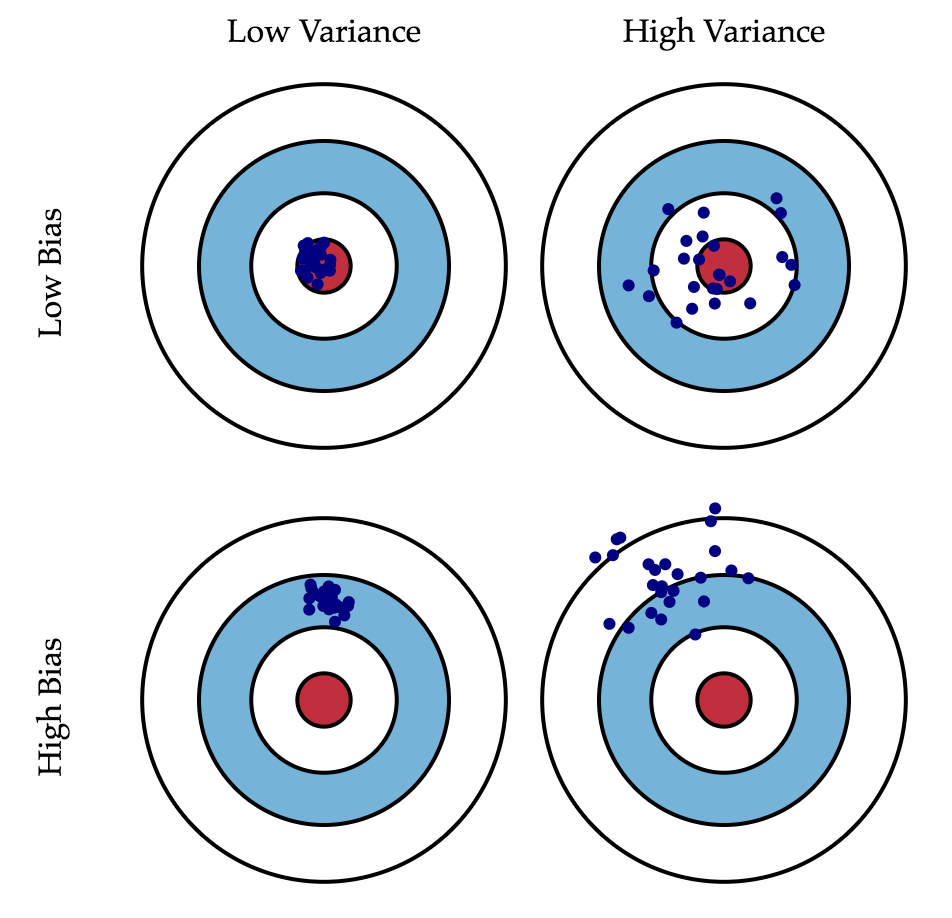
Как правило, при увеличении сложности модели (например, при увеличении количества свободных параметров) увеличивается дисперсия (разброс) оценки, но уменьшается смещение. Из-за того что тренировочный набор данных полностью запоминается вместо обобщения, небольшие изменения приводят к неожиданным результатам (переобучение). Если же модель слабая, то она не состоянии выучить закономерность, в результате выучивается что-то другое, смещенное относительно правильного решения.

Теорема Маркова-Гаусса как раз утверждает, что МНК-оценка параметров линейной модели является самой лучшей в классе несмещенных линейных оценок, то есть с наименьшей дисперсией. Это значит, что если существует какая-либо другая несмещенная модель  тоже из класса линейных моделей, то мы можем быть уверены, что
  .
.
Регуляризация линейной регрессии
Иногда бывают ситуации, когда мы намеренно увеличиваем смещенность модели ради ее стабильности, т.е. ради уменьшения дисперсии модели  . Одним из условий теоремы Маркова-Гаусса является полный столбцовый ранг матрицы . В противном случае решение МНК
  не существует, т.к. не будет существовать обратная матрица
  Другими словами, матрица
  будет сингулярна, или вырожденна. Такая задача называется некорректно поставленной. Задачу нужно скорректировать, а именно, сделать матрицу невырожденной, или регулярной (именно поэтому этот процесс называется регуляризацией). Чаще в данных мы можем наблюдать так называемую мультиколлинеарность — когда два или несколько признаков сильно коррелированы, в матрице это проявляется в виде «почти» линейной зависимости столбцов. Например, в задаче прогнозирования цены квартиры по ее параметрам «почти» линейная зависимость будет у признаков «площадь с учетом балкона» и «площадь без учета балкона». Формально для таких данных матрица будет обратима, но из-за мультиколлинеарности у матрицы некоторые собственные значения будут близки к нулю, а в обратной матрице
  появятся экстремально большие собственные значения, т.к. собственные значения обратной матрицы – это
  . Итогом такого шатания собственных значений станет нестабильная оценка параметров модели, т.е. добавление нового наблюдения в набор тренировочных данных приведёт к совершенно другому решению. Иллюстрации роста коэффициентов вы найдете в одном из наших прошлых постов. Одним из способов регуляризации является регуляризация Тихонова, которая в общем виде выглядит как добавление нового члена к среднеквадратичной ошибке:

Часто матрица Тихонова выражается как произведение некоторого числа на единичную матрицу:  . В этом случае задача минимизации среднеквадратичной ошибки становится задачей с ограничением на
  норму. Если продифференцировать новую функцию стоимости по параметрам модели, приравнять полученную функцию к нулю и выразить , то мы получим точное решение задачи.

Такая регрессия называется гребневой регрессией (ridge regression). А гребнем является как раз диагональная матрица, которую мы прибавляем к матрице , в результате получается гарантированно регулярная матрица.

Такое решение уменьшает дисперсию, но становится смещенным, т.к. минимизируется также и норма вектора параметров, что заставляет решение сдвигаться в сторону нуля. На рисунке ниже на пересечении белых пунктирных линий находится МНК-решение. Голубыми точками обозначены различные решения гребневой регрессии. Видно, что при увеличении параметра регуляризации  решение сдвигается в сторону нуля.
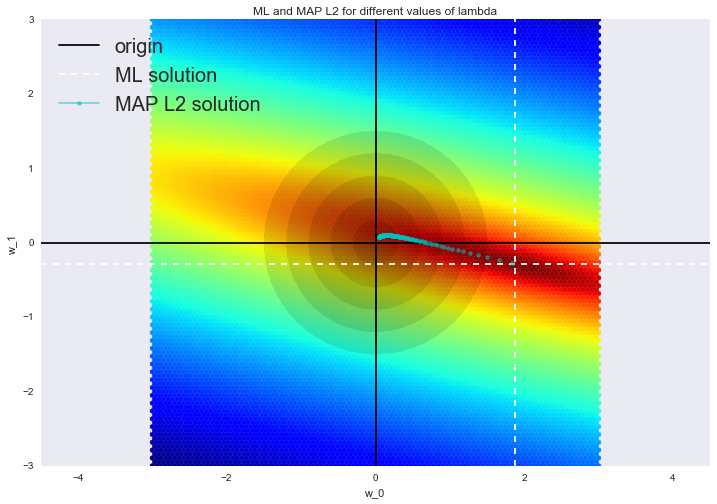
Советуем обратиться в наш прошлый пост за примером того, как регуляризация справляется с проблемой мультиколлинеарности, а также чтобы освежить в памяти еще несколько интерпретаций регуляризации.
2. Логистическая регрессия
Линейный классификатор
Основная идея линейного классификатора заключается в том, что признаковое пространство может быть разделено гиперплоскостью на две полуплоскости, в каждой из которых прогнозируется одно из двух значений целевого класса.
Если это можно сделать без ошибок, то обучающая выборка называется линейно разделимой.

Мы уже знакомы с линейной регрессией и методом наименьших квадратов. Рассмотрим задачу бинарной классификации, причем метки целевого класса обозначим «+1» (положительные примеры) и «-1» (отрицательные примеры).
Один из самых простых линейных классификаторов получается на основе регрессии вот таким образом:

где
Логистическая регрессия как линейный классификатор
Логистическая регрессия является частным случаем линейного классификатора, но она обладает хорошим «умением» – прогнозировать вероятность  отнесения примера
  к классу «+»:

Прогнозирование не просто ответа («+1» или «-1»), а именно вероятности отнесения к классу «+1» во многих задачах является очень важным бизнес-требованием. Например, в задаче кредитного скоринга, где традиционно применяется логистическая регрессия, часто прогнозируют вероятность невозврата кредита (). Клиентов, обратившихся за кредитом, сортируют по этой предсказанной вероятности (по убыванию), и получается скоркарта — по сути, рейтинг клиентов от плохих к хорошим. Ниже приведен игрушечный пример такой скоркарты.

Банк выбирает для себя порог  предсказанной вероятности невозврата кредита (на картинке –
  ) и начиная с этого значения уже не выдает кредит. Более того, можно умножить предсказанную вероятность на выданную сумму и получить матожидание потерь с клиента, что тоже будет хорошей бизнес-метрикой (Далее в комментариях специалисты по скорингу могут поправить, но главная суть примерно такая).
Итак, мы хотим прогнозировать вероятность ![$p_+ in [0,1]$](https://habrastorage.org/getpro/habr/post_images/624/c6f/a2f/624c6fa2f2f9e8ef64089d57b357b588.svg) , а пока умеем строить линейный прогноз с помощью МНК:
, а пока умеем строить линейный прогноз с помощью МНК:  . Каким образом преобразовать полученное значение в вероятность, пределы которой – [0, 1]? Очевидно, для этого нужна некоторая функция
 ![$f: mathbb{R} rightarrow [0,1].$](https://habrastorage.org/getpro/habr/post_images/1b2/b4c/9fa/1b2b4c9fa5bd7c14754664a95285bcd2.svg) В модели логистической регрессии для этого берется конкретная функция:
В модели логистической регрессии для этого берется конкретная функция:  . И сейчас разберемся, каковы для этого предпосылки.

Обозначим  вероятностью происходящего события . Тогда отношение вероятностей
  определяется из
  , а это — отношение вероятностей того, произойдет ли событие или не произойдет. Очевидно, что вероятность и отношение шансов содержат одинаковую информацию. Но в то время как находится в пределах от 0 до 1, находится в пределах от 0 до
  .
.
Если вычислить логарифм (то есть называется логарифм шансов, или логарифм отношения вероятностей), то легко заметить, что  . Его то мы и будем прогнозировать с помощью МНК.
Посмотрим, как логистическая регрессия будет делать прогноз  (пока считаем, что веса мы как-то получили (т.е. обучили модель), далее разберемся, как именно).

В правой части мы получили как раз сигмоид-функцию.
Итак, логистическая регрессия прогнозирует вероятность отнесения примера к классу «+» (при условии, что мы знаем его признаки и веса модели) как сигмоид-преобразование линейной комбинации вектора весов модели и вектора признаков примера:

Следующий вопрос: как модель обучается? Тут мы опять обращаемся к принципу максимального правдоподобия.
Принцип максимального правдоподобия и логистическая регрессия
Теперь посмотрим, как из принципа максимального правдоподобия получается оптимизационная задача, которую решает логистическая регрессия, а именно, – минимизация логистической функции потерь.
Только что мы увидели, что логистическая регрессия моделирует вероятность отнесения примера к классу «+» как

Тогда для класса «-» аналогичная вероятность:

Оба этих выражения можно ловко объединить в одно (следите за моими руками – не обманывают ли вас):

Выражение  называется отступом (margin) классификации на объекте (не путать с зазором (тоже margin), про который чаще всего говорят в контексте SVM). Если он неотрицателен, модель не ошибается на объекте , если же отрицателен – значит, класс для спрогнозирован неправильно.
Заметим, что отступ определен для объектов именно обучающей выборки, для которых известны реальные метки целевого класса  .
.
Чтобы понять, почему это мы сделали такие выводы, обратимся к геометрической интерпретации линейного классификатора. Подробно про это можно почитать в материалах Евгения Соколова.
Рекомендую решить почти классическую задачу из начального курса линейной алгебры: найти расстояние от точки с радиус-вектором  до плоскости, которая задается уравнением
Ответ


Когда получим (или посмотрим) ответ, то поймем, что чем больше по модулю выражение  , тем дальше точка находится от плоскости
Значит, выражение – это своего рода «уверенность» модели в классификации объекта :
- если отступ большой (по модулю) и положительный, это значит, что метка класса поставлена правильно, а объект находится далеко от разделяющей гиперплоскости (такой объект классифицируется уверенно). На рисунке – .
- если отступ большой (по модулю) и отрицательный, значит метка класса поставлена неправильно, а объект находится далеко от разделяющей гиперплоскости (скорее всего такой объект – аномалия, например, его метка в обучающей выборке поставлена неправильно). На рисунке – .
- если отступ малый (по модулю), то объект находится близко к разделяющей гиперплоскости, а знак отступа определяет, правильно ли объект классифицирован. На рисунке – и .
 .
. .
.
Теперь распишем правдоподобие выборки, а именно, вероятность наблюдать данный вектор  у выборки . Делаем сильное предположение: объекты приходят независимо, из одного распределения (i.i.d.). Тогда

где  – длина выборки (число строк).
Как водится, возьмем логарифм данного выражения (сумму оптимизировать намного проще, чем произведение):

То есть в даном случае принцип максимизации правдоподобия приводит к минимизации выражения

Это логистическая функция потерь, просуммированная по всем объектам обучающей выборки.
Посмотрим на новую фунцию как на функцию от отступа:  . Нарисуем ее график, а также график 1/0 функциий потерь (zero-one loss), которая просто штрафует модель на 1 за ошибку на каждом объекте (отступ отрицательный):
 ![$L_{1/0}(M) = [M < 0]$](https://habrastorage.org/getpro/habr/post_images/241/260/ede/241260ede206ec501fcc94508d08d32d.svg) .
.

Картинка отражает общую идею, что в задаче классификации, не умея напрямую минимизировать число ошибок (по крайней мере, градиентными методами это не сделать – производная 1/0 функциий потерь в нуле обращается в бесконечность), мы минимизируем некоторую ее верхнюю оценку. В данном случае это логистическая функция потерь (где логарифм двоичный, но это не принципиально), и справедливо
![$large begin{array}{rcl} mathcal{L_{1/0}} (X, vec{y}, vec{w}) &=& sum_{i=1}^{ell} [M(vec{x_i}) < 0] \ &leq& sum_{i=1}^{ell} log (1 + exp^{-y_ivec{w}^Tvec{x_i}}) \ &=& mathcal{L_{log}} (X, vec{y}, vec{w}) end{array}$](https://habrastorage.org/getpro/habr/post_images/5a6/9ad/598/5a69ad59865ad980fed636c81c7b8a68.svg)
где  – попросту число ошибок логистической регрессии с весами на выборке
  .
.
То есть уменьшая верхнюю оценку  на число ошибок классификации, мы таким образом надеемся уменьшить и само число ошибок.
-регуляризация логистических потерь
L2-регуляризация логистической регрессии устроена почти так же, как и в случае с гребневой (Ridge регрессией). Вместо функционала  минимизируется следующий:

В случае логистической регрессии принято введение обратного коэффициента регуляризации  . И тогда решением задачи будет

Далее рассмотрим пример, позволяющий интуитивно понять один из смыслов регуляризации.
3. Наглядный пример регуляризации логистической регрессии
В 1 статье уже приводился пример того, как полиномиальные признаки позволяют линейным моделям строить нелинейные разделяющие поверхности. Покажем это в картинках.
Посмотрим, как регуляризация влияет на качество классификации на наборе данных по тестированию микрочипов из курса Andrew Ng по машинному обучению.
Будем использовать логистическую регрессию с полиномиальными признаками и варьировать параметр регуляризации C.
Сначала посмотрим, как регуляризация влияет на разделяющую границу классификатора, интуитивно распознаем переобучение и недообучение.
Потом численно установим близкий к оптимальному параметр регуляризации с помощью кросс-валидации (cross-validation) и перебора по сетке (GridSearch).
Подлюкчение библиотек
from __future__ import division, print_function
# отключим всякие предупреждения Anaconda
import warnings
warnings.filterwarnings('ignore')
%matplotlib inline
from matplotlib import pyplot as plt
import seaborn as sns

import numpy as np
import pandas as pd
from sklearn.preprocessing import PolynomialFeatures
from sklearn.linear_model import LogisticRegression, LogisticRegressionCV
from sklearn.model_selection import cross_val_score, StratifiedKFold
from sklearn.model_selection import GridSearchCV
Загружаем данные с помощью метода read_csv библиотеки pandas. В этом наборе данных для 118 микрочипов (объекты) указаны результаты двух тестов по контролю качества (два числовых признака) и сказано, пустили ли микрочип в производство. Признаки уже центрированы, то есть из всех значений вычтены средние по столбцам. Таким образом, «среднему» микрочипу соответствуют нулевые значения результатов тестов.
Загрузка данных
data = pd.read_csv('../../data/microchip_tests.txt',
header=None, names = ('test1','test2','released'))
# информация о наборе данных
data.info()
<class ‘pandas.core.frame.DataFrame’>
RangeIndex: 118 entries, 0 to 117
Data columns (total 3 columns):
test1 118 non-null float64
test2 118 non-null float64
released 118 non-null int64
dtypes: float64(2), int64(1)
memory usage: 2.8 KB
Посмотрим на первые и последние 5 строк.
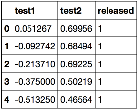
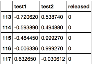
Сохраним обучающую выборку и метки целевого класса в отдельных массивах NumPy. Отобразим данные. Красный цвет соответствует бракованным чипам, зеленый – нормальным.
Код
X = data.ix[:,:2].values
y = data.ix[:,2].values
plt.scatter(X[y == 1, 0], X[y == 1, 1], c='green', label='Выпущен')
plt.scatter(X[y == 0, 0], X[y == 0, 1], c='red', label='Бракован')
plt.xlabel("Тест 1")
plt.ylabel("Тест 2")
plt.title('2 теста микрочипов')
plt.legend();
Определяем функцию для отображения разделяющей кривой классификатора
Код
def plot_boundary(clf, X, y, grid_step=.01, poly_featurizer=None):
x_min, x_max = X[:, 0].min() - .1, X[:, 0].max() + .1
y_min, y_max = X[:, 1].min() - .1, X[:, 1].max() + .1
xx, yy = np.meshgrid(np.arange(x_min, x_max, grid_step),
np.arange(y_min, y_max, grid_step))

# каждой точке в сетке [x_min, m_max]x[y_min, y_max]
# ставим в соответствие свой цвет
Z = clf.predict(poly_featurizer.transform(np.c_[xx.ravel(), yy.ravel()]))
Z = Z.reshape(xx.shape)
plt.contour(xx, yy, Z, cmap=plt.cm.Paired)
Полиномиальными признаками до степени  для двух переменных
  и
и  мы называем следующие:

Например, для  это будут следующие признаки:

Нарисовав треугольник Пифагора, Вы сообразите, сколько таких признаков будет для  и вообще для любого .
Попросту говоря, таких признаков экспоненциально много, и строить, скажем, для 100 признаков полиномиальные степени 10 может оказаться затратно (а более того, и не нужно).
Создадим объект sklearn, который добавит в матрицу полиномиальные признаки вплоть до степени 7 и обучим логистическую регрессию с параметром регуляризации  . Изобразим разделяющую границу.
Также проверим долю правильных ответов классификатора на обучающей выборке. Видим, что регуляризация оказалась слишком сильной, и модель «недообучилась». Доля правильных ответов классификатора на обучающей выборке оказалась равной 0.627.
Код
poly = PolynomialFeatures(degree=7)
X_poly = poly.fit_transform(X)
C = 1e-2
logit = LogisticRegression(C=C, n_jobs=-1, random_state=17)
logit.fit(X_poly, y)
plot_boundary(logit, X, y, grid_step=.01, poly_featurizer=poly)
plt.scatter(X[y == 1, 0], X[y == 1, 1], c='green', label='Выпущен')
plt.scatter(X[y == 0, 0], X[y == 0, 1], c='red', label='Бракован')
plt.xlabel("Тест 1")
plt.ylabel("Тест 2")
plt.title('2 теста микрочипов. Логит с C=0.01')
plt.legend();
print("Доля правильных ответов классификатора на обучающей выборке:",
round(logit.score(X_poly, y), 3))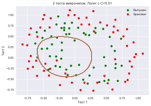
Увеличим  до 1. Тем самым мы ослабляем регуляризацию, теперь в решении значения весов логистической регрессии могут оказаться больше (по модулю), чем в прошлом случае. Теперь доля правильных ответов классификатора на обучающей выборке – 0.831.
Код
C = 1
logit = LogisticRegression(C=C, n_jobs=-1, random_state=17)
logit.fit(X_poly, y)

plot_boundary(logit, X, y, grid_step=.005, poly_featurizer=poly)

plt.scatter(X[y == 1, 0], X[y == 1, 1], c='green', label='Выпущен')
plt.scatter(X[y == 0, 0], X[y == 0, 1], c='red', label='Бракован')
plt.xlabel("Тест 1")
plt.ylabel("Тест 2")
plt.title('2 теста микрочипов. Логит с C=1')
plt.legend();

print("Доля правильных ответов классификатора на обучающей выборке:",
round(logit.score(X_poly, y), 3))
Еще увеличим – до 10 тысяч. Теперь регуляризации явно недостаточно, и мы наблюдаем переобучение. Можно заметить, что в прошлом случае (при =1 и «гладкой» границе) доля правильных ответов модели на обучающей выборке не намного ниже, чем в 3 случае, зато на новой выборке, можно себе представить, 2 модель сработает намного лучше.
Доля правильных ответов классификатора на обучающей выборке – 0.873.
Код
C = 1e4
logit = LogisticRegression(C=C, n_jobs=-1, random_state=17)
logit.fit(X_poly, y)

plot_boundary(logit, X, y, grid_step=.005, poly_featurizer=poly)

plt.scatter(X[y == 1, 0], X[y == 1, 1], c='green', label='Выпущен')
plt.scatter(X[y == 0, 0], X[y == 0, 1], c='red', label='Бракован')
plt.xlabel("Тест 1")
plt.ylabel("Тест 2")
plt.title('2 теста микрочипов. Логит с C=10k')
plt.legend();

print("Доля правильных ответов классификатора на обучающей выборке:",
round(logit.score(X_poly, y), 3))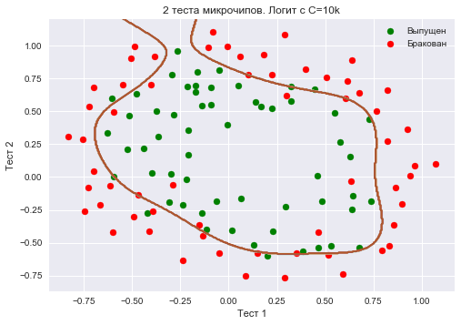
Чтоб обсудить результаты, перепишем формулу для функционала, который оптимизируется в логистической регрессии, в таком виде:

где
Промежуточные выводы:
- чем больше параметр , тем более сложные зависимости в данных может восстанавливать модель (интуитивно соответствует «сложности» модели (model capacity))
- если регуляризация слишком сильная (малые значения ), то решением задачи минимизации логистической функции потерь может оказаться то, когда многие веса занулились или стали слишком малыми. Еще говорят, что модель недостаточно «штрафуется» за ошибки (то есть в функционале «перевешивает» сумма квадратов весов, а ошибка может быть относительно большой). В таком случае модель окажется недообученной (1 случай)
- наоборот, если регуляризация слишком слабая (большие значения ), то решением задачи оптимизации может стать вектор с большими по модулю компонентами. В таком случае больший вклад в оптимизируемый функционал имеет и, вольно выражаясь, модель слишком «боится» ошибиться на объектах обучающей выборки, поэтому окажется переобученной (3 случай)
- то, какое значение выбрать, сама логистическая регрессия «не поймет» (или еще говорят «не выучит»), то есть это не может быть определено решением оптимизационной задачи, которой является логистическая регрессия (в отличие от весов ). Так же точно, дерево решений не может «само понять», какое ограничение на глубину выбрать (за один процесс обучения). Поэтому – это гиперпараметр модели, который настраивается на кросс-валидации, как и max_depth для дерева.
 «перевешивает» сумма квадратов весов, а ошибка
  может быть относительно большой). В таком случае модель окажется недообученной (1 случай)
 с большими по модулю компонентами. В таком случае больший вклад в оптимизируемый функционал
 Настройка параметра регуляризации
Теперь найдем оптимальное (в данном примере) значение параметра регуляризации . Сделать это можно с помощью LogisticRegressionCV – перебора параметров по сетке с последующей кросс-валидацией. Этот класс создан специально для логистической регрессии (для нее известны эффективные алгоритмы перебора параметров), для произвольной модели мы бы использовали GridSearchCV, RandomizedSearchCV или, например, специальные алгоритмы оптимизации гиперпараметров, реализованные в hyperopt.
Код
skf = StratifiedKFold(n_splits=5, shuffle=True, random_state=17)

c_values = np.logspace(-2, 3, 500)

logit_searcher = LogisticRegressionCV(Cs=c_values, cv=skf, verbose=1, n_jobs=-1)
logit_searcher.fit(X_poly, y)
Посмотрим, как качество модели (доля правильных ответов на обучающей и валидационной выборках) меняется при изменении гиперпараметра .

Выделим участок с «лучшими» значениями C.

Как мы помним, такие кривые называются валидационными, раньше мы их строили вручную, но в sklearn для них их построения есть специальные методы, которые мы тоже сейчас будем использовать.
Анализ отзывов IMDB к фильмам
Будем решать задачу бинарной классификации отзывов IMDB к фильмам. Имеется обучающая выборка с размеченными отзывами, по 12500 отзывов известно, что они хорошие, еще про 12500 – что они плохие. Здесь уже не так просто сразу приступить к машинному обучению, потому что готовой матрицы нет – ее надо приготовить. Будем использовать самый простой подход – мешок слов («Bag of words»). При таком подходе признаками отзыва будут индикаторы наличия в нем каждого слова из всего корпуса, где корпус – это множество всех отзывов. Идея иллюстрируется картинкой
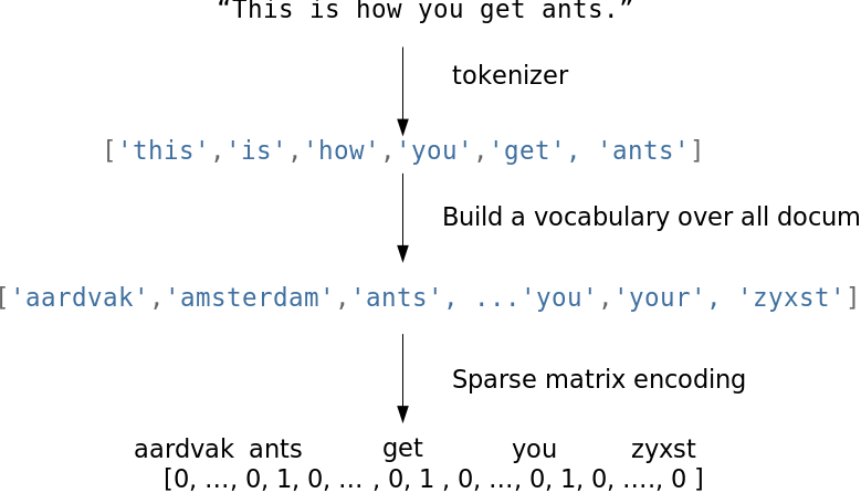
Импорт библиотек и загрузка данных
from __future__ import division, print_function
# отключим всякие предупреждения Anaconda
import warnings
warnings.filterwarnings('ignore')
import numpy as np
import matplotlib.pyplot as plt
%matplotlib inline
import seaborn as sns
import numpy as np
from sklearn.datasets import load_files
from sklearn.feature_extraction.text import CountVectorizer, TfidfTransformer, TfidfVectorizer
from sklearn.linear_model import LogisticRegression
from sklearn.svm import LinearSVC
Загрузим данные отсюда. В обучающей и тестовой выборках по 12500 тысяч хороших и плохих отзывов к фильмам.
reviews_train = load_files("YOUR PATH")
text_train, y_train = reviews_train.data, reviews_train.target
print("Number of documents in training data: %d" % len(text_train))
print(np.bincount(y_train))# поменяйте путь к файлу
reviews_test = load_files("YOUR PATH")
text_test, y_test = reviews_test.data, reviews_test.target
print("Number of documents in test data: %d" % len(text_test))
print(np.bincount(y_test))Пример плохого отзыва:
‘Words can’t describe how bad this movie is. I can’t explain it by writing only. You have too see it for yourself to get at grip of how horrible a movie really can be. Not that I recommend you to do that. There are so many clichxc3xa9s, mistakes (and all other negative things you can imagine) here that will just make you cry. To start with the technical first, there are a LOT of mistakes regarding the airplane. I won’t list them here, but just mention the coloring of the plane. They didn’t even manage to show an airliner in the colors of a fictional airline, but instead used a 747 painted in the original Boeing livery. Very bad. The plot is stupid and has been done many times before, only much, much better. There are so many ridiculous moments here that i lost count of it really early. Also, I was on the bad guys’ side all the time in the movie, because the good guys were so stupid. «Executive Decision» should without a doubt be you’re choice over this one, even the «Turbulence»-movies are better. In fact, every other movie in the world is better than this one.’
Пример хорошего отзыва:
‘Everyone plays their part pretty well in this «little nice movie». Belushi gets the chance to live part of his life differently, but ends up realizing that what he had was going to be just as good or maybe even better. The movie shows us that we ought to take advantage of the opportunities we have, not the ones we do not or cannot have. If U can get this movie on video for around $10, itxc2xb4d be an investment!’
Простой подсчет слов
Составим словарь всех слов с помощью CountVectorizer. Всего в выборке 74849 уникальных слов. Если посмотреть на примеры полученных «слов» (лучше их называть токенами), то можно увидеть, что многие важные этапы обработки текста мы тут пропустили (автоматическая обработка текстов – это могло бы быть темой отдельной серии статей).
Код
cv = CountVectorizer()
cv.fit(text_train)

print(len(cv.vocabulary_)) #74849
print(cv.get_feature_names()[:50])
print(cv.get_feature_names()[50000:50050])[’00’, ‘000’, ‘0000000000001’, ‘00001’, ‘00015’, ‘000s’, ‘001’, ‘003830’, ‘006’, ‘007’, ‘0079’, ‘0080’, ‘0083’, ‘0093638’, ’00am’, ’00pm’, ’00s’, ’01’, ’01pm’, ’02’, ‘020410’, ‘029’, ’03’, ’04’, ‘041’, ’05’, ‘050’, ’06’, ’06th’, ’07’, ’08’, ‘087’, ‘089’, ’08th’, ’09’, ‘0f’, ‘0ne’, ‘0r’, ‘0s’, ’10’, ‘100’, ‘1000’, ‘1000000’, ‘10000000000000’, ‘1000lb’, ‘1000s’, ‘1001’, ‘100b’, ‘100k’, ‘100m’]
[‘pincher’, ‘pinchers’, ‘pinches’, ‘pinching’, ‘pinchot’, ‘pinciotti’, ‘pine’, ‘pineal’, ‘pineapple’, ‘pineapples’, ‘pines’, ‘pinet’, ‘pinetrees’, ‘pineyro’, ‘pinfall’, ‘pinfold’, ‘ping’, ‘pingo’, ‘pinhead’, ‘pinheads’, ‘pinho’, ‘pining’, ‘pinjar’, ‘pink’, ‘pinkerton’, ‘pinkett’, ‘pinkie’, ‘pinkins’, ‘pinkish’, ‘pinko’, ‘pinks’, ‘pinku’, ‘pinkus’, ‘pinky’, ‘pinnacle’, ‘pinnacles’, ‘pinned’, ‘pinning’, ‘pinnings’, ‘pinnochio’, ‘pinnocioesque’, ‘pino’, ‘pinocchio’, ‘pinochet’, ‘pinochets’, ‘pinoy’, ‘pinpoint’, ‘pinpoints’, ‘pins’, ‘pinsent’]
Закодируем предложения из текстов обучающей выборки индексами входящих слов. Используем разреженный формат. Преобразуем так же тестовую выборку.
X_train = cv.transform(text_train)
X_test = cv.transform(text_test)
Обучим логистическую регрессию и посмотрим на доли правильных ответов на обучающей и тестовой выборках. Получается, на тестовой выборке мы правильно угадываем тональность примерно 86.7% отзывов.
Код
%%time
logit = LogisticRegression(n_jobs=-1, random_state=7)
logit.fit(X_train, y_train)
print(round(logit.score(X_train, y_train), 3), round(logit.score(X_test, y_test), 3))
Коэффициенты модели можно красиво отобразить.
Код визуализации коэффициентов модели
def visualize_coefficients(classifier, feature_names, n_top_features=25):
# get coefficients with large absolute values
coef = classifier.coef_.ravel()
positive_coefficients = np.argsort(coef)[-n_top_features:]
negative_coefficients = np.argsort(coef)[:n_top_features]
interesting_coefficients = np.hstack([negative_coefficients, positive_coefficients])
# plot them
plt.figure(figsize=(15, 5))
colors = ["red" if c < 0 else "blue" for c in coef[interesting_coefficients]]
plt.bar(np.arange(2 * n_top_features), coef[interesting_coefficients], color=colors)
feature_names = np.array(feature_names)
plt.xticks(np.arange(1, 1 + 2 * n_top_features), feature_names[interesting_coefficients], rotation=60, ha="right");
def plot_grid_scores(grid, param_name):
plt.plot(grid.param_grid[param_name], grid.cv_results_['mean_train_score'],
color='green', label='train')
plt.plot(grid.param_grid[param_name], grid.cv_results_['mean_test_score'],
color='red', label='test')
plt.legend();
visualize_coefficients(logit, cv.get_feature_names())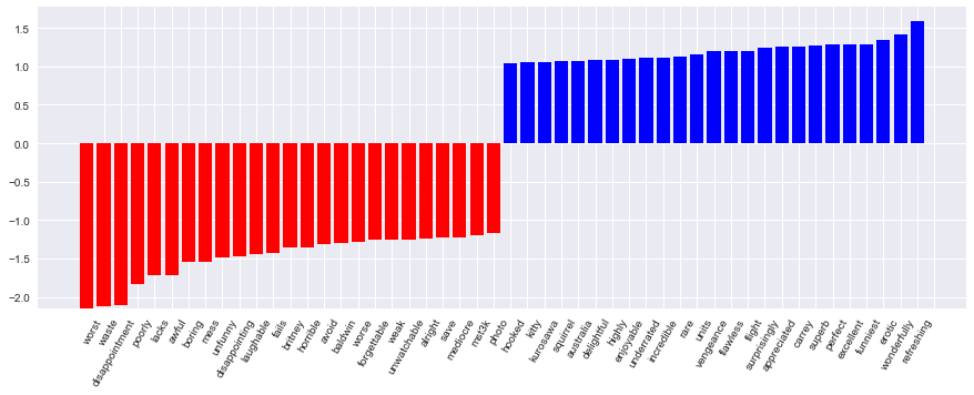
Подберем коэффициент регуляризации для логистической регрессии. Используем sklearn.pipeline, поскольку CountVectorizer правильно применять только на тех данных, на которых в текущий момент обучается модель (чтоб не «подсматривать» в тестовую выборку и не считать по ней частоты вхождения слов). В данном случае pipeline задает последовательность действий: применить CountVectorizer, затем обучить логистическую регрессию. Так мы поднимаем долю правильных ответов до 88.5% на кросс-валидации и 87.9% – на отложенной выборке.
Код
from sklearn.pipeline import make_pipeline

text_pipe_logit = make_pipeline(CountVectorizer(),
LogisticRegression(n_jobs=-1, random_state=7))

text_pipe_logit.fit(text_train, y_train)
print(text_pipe_logit.score(text_test, y_test))

from sklearn.model_selection import GridSearchCV

param_grid_logit = {'logisticregression__C': np.logspace(-5, 0, 6)}
grid_logit = GridSearchCV(text_pipe_logit, param_grid_logit, cv=3, n_jobs=-1)

grid_logit.fit(text_train, y_train)
grid_logit.best_params_, grid_logit.best_score_
plot_grid_scores(grid_logit, 'logisticregression__C')
grid_logit.score(text_test, y_test)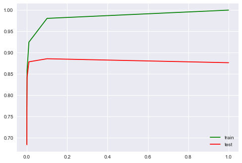
Теперь то же самое, но со случайным лесом. Видим, что с логистической регрессией мы достигаем большей доли правильных ответов меньшими усилиями. Лес работает дольше, на отложенной выборке 85.5% правильных ответов.
Код для обучения случайного леса
from sklearn.ensemble import RandomForestClassifier
forest = RandomForestClassifier(n_estimators=200, n_jobs=-1, random_state=17)
forest.fit(X_train, y_train)
print(round(forest.score(X_test, y_test), 3))
XOR-проблема
Теперь рассмотрим пример, где линейные модели справляются хуже.
Линейные методы классификации строят все же очень простую разделяющую поверхность – гиперплоскость. Самый известный игрушечный пример, в котором классы нельзя без ошибок поделить гиперплоскостью (то есть прямой, если это 2D), получил имя «the XOR problem».
XOR – это «исключающее ИЛИ», булева функция со следующей таблицей истинности:
XOR дал имя простой задаче бинарной классификации, в которой классы представлены вытянутыми по диагоналям и пересекающимися облаками точек.
Код, рисующий следующие 3 картинки
# порождаем данные
rng = np.random.RandomState(0)
X = rng.randn(200, 2)
y = np.logical_xor(X[:, 0] > 0, X[:, 1] > 0)
plt.scatter(X[:, 0], X[:, 1], s=30, c=y, cmap=plt.cm.Paired);def plot_boundary(clf, X, y, plot_title):
xx, yy = np.meshgrid(np.linspace(-3, 3, 50),
np.linspace(-3, 3, 50))
clf.fit(X, y)
# plot the decision function for each datapoint on the grid
Z = clf.predict_proba(np.vstack((xx.ravel(), yy.ravel())).T)[:, 1]
Z = Z.reshape(xx.shape)
image = plt.imshow(Z, interpolation='nearest',
extent=(xx.min(), xx.max(), yy.min(), yy.max()),
aspect='auto', origin='lower', cmap=plt.cm.PuOr_r)
contours = plt.contour(xx, yy, Z, levels=[0], linewidths=2,
linetypes='--')
plt.scatter(X[:, 0], X[:, 1], s=30, c=y, cmap=plt.cm.Paired)
plt.xticks(())
plt.yticks(())
plt.xlabel(r'<!-- math><img src="https://habrastorage.org/getpro/habr/post_images/736/3ed/315/7363ed3150ecffdf235171aaa9ea4160.svg" alt="$x_1$" data-tex="inline" /></math -->')
plt.ylabel(r'<!-- math><img src="https://habrastorage.org/getpro/habr/post_images/911/1e6/994/9111e69946e97ffe28324cbae67a9269.svg" alt="$x_2$" data-tex="inline" /></math -->')
plt.axis([-3, 3, -3, 3])
plt.colorbar(image)
plt.title(plot_title, fontsize=12);plot_boundary(LogisticRegression(), X, y,
"Logistic Regression, XOR problem")from sklearn.preprocessing import PolynomialFeatures
from sklearn.pipeline import Pipelinelogit_pipe = Pipeline([('poly', PolynomialFeatures(degree=2)),
('logit', LogisticRegression())])plot_boundary(logit_pipe, X, y,
"Logistic Regression + quadratic features. XOR problem")
Очевидно, нельзя провести прямую так, чтобы без ошибок отделить один класс от другого. Поэтому логистическая регрессия плохо справляется с такой задачей.
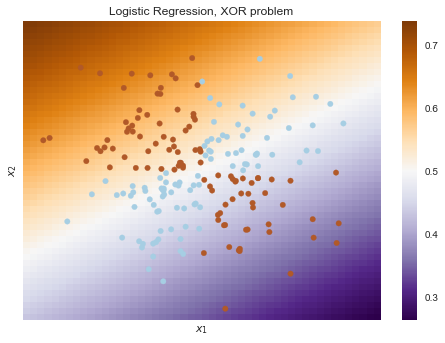
А вот если на вход подать полиномиальные признаки, в данном случае до 2 степени, то проблема решается.
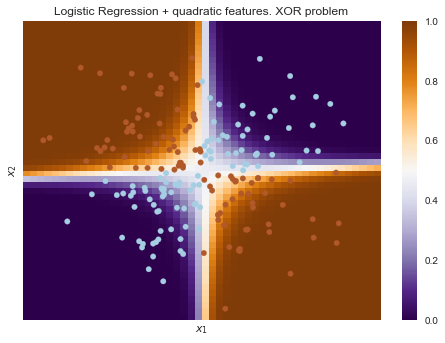
Здесь логистическая регрессия все равно строила гиперплоскость, но в 6-мерном пространстве признаков  и
и  . В проекции на исходное пространство признаков
  граница получилась нелинейной.
На практике полиномиальные признаки действительно помогают, но строить их явно – вычислительно неэффективно. Гораздо быстрее работает SVM с ядровым трюком. При таком подходе в пространстве высокой размерности считается только расстояние между объектами (задаваемое функцией-ядром), а явно плодить комбинаторно большое число признаков не приходится. Про это подробно можно почитать в курсе Евгения Соколова (математика уже серьезная).
5. Кривые валидации и обучения
Мы уже получили представление о проверке модели, кросс-валидации и регуляризации.
Теперь рассмотрим главный вопрос:
Если качество модели нас не устраивает, что делать?
- Сделать модель сложнее или упростить?
- Добавить больше признаков?
- Или нам просто нужно больше данных для обучения?
Ответы на данные вопросы не всегда лежат на поверхности. В частности, иногда использование более сложной модели приведет к ухудшению показателей. Либо добавление наблюдений не приведет к ощутимым изменениям. Способность принять правильное решение и выбрать правильный способ улучшения модели, собственно говоря, и отличает хорошего специалиста от плохого.
Будем работать со знакомыми данными по оттоку клиентов телеком-оператора.
Импорт библиотек и чтение данных
from __future__ import division, print_function
# отключим всякие предупреждения Anaconda
import warnings
warnings.filterwarnings('ignore')
%matplotlib inline
from matplotlib import pyplot as plt
import seaborn as sns
import numpy as np
import pandas as pd
from sklearn.preprocessing import PolynomialFeatures
from sklearn.pipeline import Pipeline
from sklearn.preprocessing import StandardScaler
from sklearn.linear_model import LogisticRegression, LogisticRegressionCV, SGDClassifier
from sklearn.model_selection import validation_curve
data = pd.read_csv('../../data/telecom_churn.csv').drop('State', axis=1)
data['International plan'] = data['International plan'].map({'Yes': 1, 'No': 0})
data['Voice mail plan'] = data['Voice mail plan'].map({'Yes': 1, 'No': 0})
y = data['Churn'].astype('int').values
X = data.drop('Churn', axis=1).valuesЛогистическую регрессию будем обучать стохастическим градиентным спуском. Пока объясним это тем, что так быстрее, но далее в программе у нас отдельная статья про это дело. Построим валидационные кривые, показывающие, как качество (ROC AUC) на обучающей и проверочной выборке меняется с изменением параметра регуляризации.
Код
alphas = np.logspace(-2, 0, 20)
sgd_logit = SGDClassifier(loss='log', n_jobs=-1, random_state=17)
logit_pipe = Pipeline([('scaler', StandardScaler()), ('poly', PolynomialFeatures(degree=2)),
('sgd_logit', sgd_logit)])
val_train, val_test = validation_curve(logit_pipe, X, y,
'sgd_logit__alpha', alphas, cv=5,
scoring='roc_auc')

def plot_with_err(x, data, **kwargs):
mu, std = data.mean(1), data.std(1)
lines = plt.plot(x, mu, '-', **kwargs)
plt.fill_between(x, mu - std, mu + std, edgecolor='none',
facecolor=lines[0].get_color(), alpha=0.2)

plot_with_err(alphas, val_train, label='training scores')
plot_with_err(alphas, val_test, label='validation scores')
plt.xlabel(r'$alpha$'); plt.ylabel('ROC AUC')
plt.legend();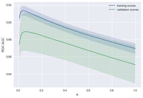
Тенденция видна сразу, и она очень часто встречается.
-
Для простых моделей тренировочная и валидационная ошибка находятся где-то рядом, и они велики. Это говорит о том, что модель недообучилась: то есть она не имеет достаточное кол-во параметров.
- Для сильно усложненных моделей тренировочная и валидационная ошибки значительно отличаются. Это можно объяснить переобучением: когда параметров слишком много либо не хватает регуляризации, алгоритм может «отвлекаться» на шум в данных и упускать основной тренд.
Сколько нужно данных?
Известно, что чем больше данных использует модель, тем лучше. Но как нам понять в конкретной ситуации, помогут ли новые данные? Скажем, целесообразно ли нам потратить N$ на труд асессоров, чтобы увеличить выборку вдвое?
Поскольку новых данных пока может и не быть, разумно поварьировать размер имеющейся обучающей выборки и посмотреть, как качество решения задачи зависит от объема данных, на котором мы обучали модель. Так получаются кривые обучения (learning curves).
Идея простая: мы отображаем ошибку как функцию от количества примеров, используемых для обучения. При этом параметры модели фиксируются заранее.
Давайте посмотрим, что мы получим для линейной модели. Коэффициент регуляризации выставим большим.
Код
from sklearn.model_selection import learning_curve

def plot_learning_curve(degree=2, alpha=0.01):
train_sizes = np.linspace(0.05, 1, 20)
logit_pipe = Pipeline([('scaler', StandardScaler()), ('poly', PolynomialFeatures(degree=degree)),
('sgd_logit', SGDClassifier(n_jobs=-1, random_state=17, alpha=alpha))])
N_train, val_train, val_test = learning_curve(logit_pipe,
X, y, train_sizes=train_sizes, cv=5,
scoring='roc_auc')
plot_with_err(N_train, val_train, label='training scores')
plot_with_err(N_train, val_test, label='validation scores')
plt.xlabel('Training Set Size'); plt.ylabel('AUC')
plt.legend()

plot_learning_curve(degree=2, alpha=10)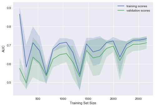
Типичная ситуация: для небольшого объема данных ошибки на обучающей выборке и в процессе кросс-валидации довольно сильно отличаются, что указывает на переобучение. Для той же модели, но с большим объемом данных ошибки «сходятся», что указывается на недообучение.
Если добавить еще данные, ошибка на обучающей выборке не будет расти, но с другой стороны, ошибка на тестовых данных не будет уменьшаться.
Получается, ошибки «сошлись», и добавление новых данных не поможет. Собственно, это случай – самый интересный для бизнеса. Возможна ситуация, когда мы увеличиваем выборку в 10 раз. Но если не менять сложность модели, это может и не помочь. То есть стратегия «настроил один раз – дальше использую 10 раз» может и не работать.
Что будет, если изменить коэффициент регуляризации (уменьшить до 0.05)?
Видим хорошую тенденцию – кривые постепенно сходятся, и если дальше двигаться направо (добавлять в модель данные), можно еще повысить качество на валидации.

А если усложнить модель ещё больше ( )?
)?
Проявляется переобучение – AUC падает как на обучении, так и на валидации.
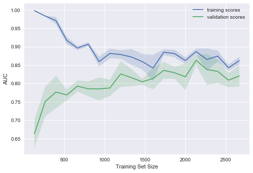
Строя подобные кривые, можно понять, в какую сторону двигаться, и как правильно настроить сложность модели на новых данных.
Выводы по кривым валидации и обучения
- Ошибка на обучающей выборке сама по себе ничего не говорит о качестве модели
- Кросс-валидационная ошибка показывает, насколько хорошо модель подстраивается под данные (имеющийся тренд в данных), сохраняя при этом способность обобщения на новые данные
- Валидационная кривая представляет собой график, показывающий результат на тренировочной и валидационной выборке в зависимости от сложности модели:
- если две кривые распологаются близко, и обе ошибки велики, — это признак недообучения
- если две кривые далеко друг от друга, — это показатель переобучения
- Кривая обучения — это график, показывающий результаты на валидации и тренировочной подвыборке в зависимости от количества наблюдений:
- если кривые сошлись друг к другу, добавление новых данных не поможет – надо менять сложность модели
- если кривые еще не сошлись, добавление новых данных может улучшить результат.
6. Плюсы и минусы линейных моделей в задачах машинного обучения
Плюсы:
Минусы:
- Плохо работают в задачах, в которых зависимость ответов от признаков сложная, нелинейная
- На практике предположения теоремы Маркова-Гаусса почти никогда не выполняются, поэтому чаще линейные методы работают хуже, чем, например, SVM и ансамбли (по качеству решения задачи классификации/регрессии)
7. Домашнее задание № 4
В этот раз задание большое, из двух частей – Часть 1 и Часть 2. Надо по инструкциям повторить базовые решения в двух соревнованиях Kaggle Inclass.
Ответы надо заполнить в веб-форме. Максимум за задание – 18 баллов. Дедлайн – 27 марта 23:59 UTC+3.
Соревнования Kaggle Inclass в нашем курсе
Теперь официально представляем 2 соревнования, результаты которых будут учитываться в рейтинге нашего курса:
- Первое «Прогноз популярности статьи на Хабре»
- Второе «Идентификация взломщика по последовательности переходов по сайтам».
Подробно про задачи написано на соответствующих страницах соревнований.
За каждое из соревнований можно получить до 40 баллов. Формула расчета числа баллов:  , где
, где  – место участника в приватном рейтинге,
  – число участников, побивших все бенчмарки в приватном рейтинге (еще могут добавиться новые бенчмарки) и чье решение удовлетворяет правилам соревнования. Соревнования открыты в течение всего курса.
8. Полезные ресурсы
- Основательный обзор классики машинного обучения и, конечно же, линейных моделей сделан в книге «Deep Learning» (I. Goodfellow, Y. Bengio, A. Courville, 2016);
- Реализация многих алгоритмов машинного обучения с нуля – репозиторий rushter. Рекомендуем изучить реализацию логистической регрессии;
- Курс Евгения Соколова по машинному обучению (материалы на GitHub). Хорошая теория, нужна неплохая математическая подготовка;
- Курс Дмитрия Ефимова на GitHub (англ.). Тоже очень качественные материалы.
Статья написана в соавторстве с mephistopheies (Павлом Нестеровым). Авторы домашнего задания – aiho (Ольга Дайховская) и das19 (Юрий Исаков). Благодарю bauchgefuehl (Анастасию Манохину) за редактирование.