
Какое животное изображено на флаге и гербе Челябинска? Какая планета расположена между Землёй и Юпитером? Оттенок какого цвета называется кардинал? Удовлетворите свою любознательность и проявите эрудицию, ответив на 15/15 вопросов теста. Удачи!
Результаты теста вы узнаете в конце. Пишите в комментариях, на сколько вопросов вы ответили! А какие вопросы вызвали затруднения?
Оттенок какого цвета называется кардинал?
Красного
Чёрного
Белого
Синего
Верно!Неверно!
Кардинал — яркий оттенок красного, названный так оттого, что в него были окрашены рясы кардиналов. Из-за окраски в этот цвет имя «кардинал» получил род птиц. Первое упоминание слова в качестве обозначения цвета в английском языке относится к 1698 году.
Какое название носит усадьба Льва Толстого, в которой он написал свои основные произведения?
Ясная Поляна
Красная Поляна
Тихая Поляна
Солнечная Поляна
Верно!Неверно!
Ясная Поляна — усадьба в Щёкинском районе Тульской области (в 14 км к юго-западу от Тулы), основанная в XVII веке и принадлежавшая сначала роду Карцевых, затем роду Волконских и Толстых.
Какая планета расположена между Землёй и Юпитером?
Верно!Неверно!
Начиная от Солнца планеты нашей солнечной системы расположены в таком порядке: Меркурий, Венера, Земля, Марс, Юпитер, Сатурн, Уран, Нептун.
К какому виду спорта относится натурбан?
Велоспорт
Конный спорт
Санный спорт
Акробатика
Верно!Неверно!
Натурбан (нем. die Naturbahn «естественная трасса») — дисциплина санного спорта, заключающаяся в спуске на скорость на санях по естественной трассе. Как и в спуске по искусственным (санно-бобслейным) трассам соревнования проводятся у мужчин на санях-одиночке и санях-двойке, у женщин на санях-одиночке.
Какое животное изображено на флаге и гербе Челябинска?
Верно!Неверно!
Главной геральдической фигурой флага и герба Челябинска является навьюченный жёлтый (золотой) верблюд в знак того, что по территории современного Челябинска проходили важные торговые пути.
Как звали американскую школьницу, написавшую письмо Андропову в самый разгар холодной войны и посетившую СССР?
Анджела Дэвис
Джессика Дуброфф
Саманта Смит
Анна Франк
Верно!Неверно!
Саманта Рид Смит — американская школьница из штата Мэн, ставшая всемирно известной благодаря переписке с Юрием Андроповым, только что ставшим генеральным секретарём ЦК КПСС, во время холодной войны.
Какая часть зрительного зала в театре расположена выше остальных?
Бенуар
Амфитеатр
Бельэтаж
Партер
Верно!Неверно!
Бельэтаж (от фр. bel «красивый», «прекрасный» и étage «этаж», «ярус») в зрительном зале — второй этаж сразу после бенуара, расположенный ниже нумерованных ярусов и амфитеатра. Это первый этаж с балконами, последующие этажи с балконами начинают нумерацию с единицы — первый ярус, второй ярус.
Под каким названием известно лекарственное средство из нашатырного спирта, масла семян аниса и экстракта солодки?
Капли египетского фараона
Капли английской королевы
Капли датского короля
Капли русского царя
Верно!Неверно!
Капли датского короля — устаревший вариант грудного эликсира. Вплоть до начала XX века применялось сходное средство под названием «капли датского короля». Его рецепт был впервые опубликован в 1772 году и включал нашатырно-анисовые капли, лакричный экстракт и укропную воду. Подобный рецепт действительно применялся в Дании ещё с конца XVII века, и носил название «Капли короля», потому что по поверию, он «мог вылечить больного от смерти».
В какой стране находится древний город Петра, привлекающий множество туристов?
Верно!Неверно!
Петра — древний город, столица Идумеи (Эдома), позже столица Набатейского царства. Сами набатеи называли свой город Rqm (Ракму). Расположен на территории современной Иордании, на высоте более 900 м над уровнем моря и 660 м над окружающей местностью, в долине Аравы, в узком каньоне Сик. В наши дни около полумиллиона туристов приезжают в Иорданию каждый год, чтобы посмотреть на Петру, строения которой свидетельствуют о её славном прошлом.
Каким словом называется отклонение от нормы, ошибки, погрешности?
Агломерация
Абстрагирование
Абстиненция
Аберрация
Верно!Неверно!
Аберрация — отклонение от нормы; ошибки, нарушения, погрешности (лат. aberratio «заблуждение, уклонение, удаление, отвлечение» ← aberrare «удаляться, отклоняться» ← ab- «от» + errare «блуждать, заблуждаться; ошибаться; колебаться»).
Какое из перечисленных морей почти всё покрыто водорослями, давшими ему название?
Балеарское море
Саргассово море
Ваттовое море
Левантийское море
Верно!Неверно!
Большие скопления плавучей бурой водоросли — саргассы, в пределах моря её запас оценивается в 4—11 млн тонн. Их обилие связано с наличием в Саргассовом море зоны схождения поверхностных течений. Здесь обитают многочисленные и разнообразные животные, частью свободноплавающие (макрелевые, летучие рыбы, морская игла, крабы, морские черепахи и др.), частью прикреплённые к водорослям (актинии, мшанки и др.).
Как в русских и легендах звали райскую птицу с головой и руками девы?
Алкимеда
Алкиона
Алконост
Алконавт
Верно!Неверно!
Алконост (от греч. «зимородок») — в русском искусстве и легендах райская птица с головой и руками девы. Часто упоминается и изображается вместе с другой райской птицей Сирин. Образ Алконоста восходит к греческому мифу о девушке Алкионе, превращённой богами в зимородка. Название и образ её, впервые появившиеся в переводных памятниках, являются результатом недоразумения: вероятно, при переписывании «Шестоднева» Иоанна Болгарского, где речь идёт о зимородке — алкионе слова славянского текста «алкионъ есть птица морская» превратилось в «алконостъ».
Кто из этих актёров не воплощал Винсента ван Гога в кино?
Кирк Дуглас
Райан Гослинг
Бенедикт Камбербэтч
Уиллем Дефо
Верно!Неверно!
Кирк Дуглас сыграл Ван Гога в фильме «Жажда жизни» (1956), Уиллем Дефо — в фильме «Ван Гог. На пороге вечности» (2018), а Бенедикт Камбербэтч — в фильме для ТВ «Ван Гог: Портрет, написанный словами» (2010).
Как называют брата жены?
Верно!Неверно!
Родного брата жены называют шурином.
В какой стране появились в продаже первые резиновые калоши?
Верно!Неверно!
Первые резиновые калоши появились в продаже в Бостоне 12 февраля 1831 года.
Тест на эрудицию: 15 заковыристых вопросов для самых любознательных






Подписывайтесь на нас в Дзен’е, чтобы не пропускать новые публикации!

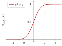
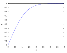
Cumulative probability of a normal distribution with expected value 0 and standard deviation 1
In statistics, the standard deviation is a measure of the amount of variation or dispersion of a set of values.[1] A low standard deviation indicates that the values tend to be close to the mean (also called the expected value) of the set, while a high standard deviation indicates that the values are spread out over a wider range.
Standard deviation may be abbreviated SD, and is most commonly represented in mathematical texts and equations by the lower case Greek letter σ (sigma), for the population standard deviation, or the Latin letter s, for the sample standard deviation.
The standard deviation of a random variable, sample, statistical population, data set, or probability distribution is the square root of its variance. It is algebraically simpler, though in practice less robust, than the average absolute deviation.[2][3] A useful property of the standard deviation is that, unlike the variance, it is expressed in the same unit as the data.
The standard deviation of a population or sample and the standard error of a statistic (e.g., of the sample mean) are quite different, but related. The sample mean’s standard error is the standard deviation of the set of means that would be found by drawing an infinite number of repeated samples from the population and computing a mean for each sample. The mean’s standard error turns out to equal the population standard deviation divided by the square root of the sample size, and is estimated by using the sample standard deviation divided by the square root of the sample size. For example, a poll’s standard error (what is reported as the margin of error of the poll), is the expected standard deviation of the estimated mean if the same poll were to be conducted multiple times. Thus, the standard error estimates the standard deviation of an estimate, which itself measures how much the estimate depends on the particular sample that was taken from the population.
In science, it is common to report both the standard deviation of the data (as a summary statistic) and the standard error of the estimate (as a measure of potential error in the findings). By convention, only effects more than two standard errors away from a null expectation are considered «statistically significant», a safeguard against spurious conclusion that is really due to random sampling error.
When only a sample of data from a population is available, the term standard deviation of the sample or sample standard deviation can refer to either the above-mentioned quantity as applied to those data, or to a modified quantity that is an unbiased estimate of the population standard deviation (the standard deviation of the entire population).
Basic examples[edit]
Population standard deviation of grades of eight students[edit]
Suppose that the entire population of interest is eight students in a particular class. For a finite set of numbers, the population standard deviation is found by taking the square root of the average of the squared deviations of the values subtracted from their average value. The marks of a class of eight students (that is, a statistical population) are the following eight values:

These eight data points have the mean (average) of 5:

First, calculate the deviations of each data point from the mean, and square the result of each:
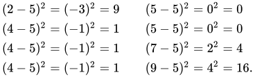
The variance is the mean of these values:

and the population standard deviation is equal to the square root of the variance:

This formula is valid only if the eight values with which we began form the complete population. If the values instead were a random sample drawn from some large parent population (for example, they were 8 students randomly and independently chosen from a class of 2 million), then one divides by 7 (which is n − 1) instead of 8 (which is n) in the denominator of the last formula, and the result is  In that case, the result of the original formula would be called the sample standard deviation and denoted by s instead of
  Dividing by n − 1 rather than by n gives an unbiased estimate of the variance of the larger parent population. This is known as Bessel’s correction.[4][5] Roughly, the reason for it is that the formula for the sample variance relies on computing differences of observations from the sample mean, and the sample mean itself was constructed to be as close as possible to the observations, so just dividing by n would underestimate the variability.
Standard deviation of average height for adult men[edit]
If the population of interest is approximately normally distributed, the standard deviation provides information on the proportion of observations above or below certain values. For example, the average height for adult men in the United States is about 70 inches, with a standard deviation of around 3 inches. This means that most men (about 68%, assuming a normal distribution) have a height within 3 inches of the mean (67–73 inches) – one standard deviation – and almost all men (about 95%) have a height within 6 inches of the mean (64–76 inches) – two standard deviations. If the standard deviation were zero, then all men would be exactly 70 inches tall. If the standard deviation were 20 inches, then men would have much more variable heights, with a typical range of about 50–90 inches. Three standard deviations account for 99.73% of the sample population being studied, assuming the distribution is normal or bell-shaped (see the 68–95–99.7 rule, or the empirical rule, for more information).
Definition of population values[edit]
Let μ be the expected value (the average) of random variable X with density f(x):
![{displaystyle mu equiv operatorname {E} [X]=int _{-infty }^{+infty }xf(x),mathrm {d} x}](https://wikimedia.org/api/rest_v1/media/math/render/svg/fb2a61843da0d05619c0dd691dbf3fe315b395ad)
The standard deviation σ of X is defined as
![{displaystyle sigma equiv {sqrt {operatorname {E} left[(X-mu )^{2}right]}}={sqrt {int _{-infty }^{+infty }(x-mu )^{2}f(x),mathrm {d} x}},}](https://wikimedia.org/api/rest_v1/media/math/render/svg/e3a1cfef8ad100fbcae387d9581763f0b389bbc3)
which can be shown to equal ![{textstyle {sqrt {operatorname {E} left[X^{2}right]-(operatorname {E} [X])^{2}}}.}](https://wikimedia.org/api/rest_v1/media/math/render/svg/e2dd8d466c3ecb05713377fefcb7e7f787b29ce7)
Using words, the standard deviation is the square root of the variance of X.
The standard deviation of a probability distribution is the same as that of a random variable having that distribution.
Not all random variables have a standard deviation. If the distribution has fat tails going out to infinity, the standard deviation might not exist, because the integral might not converge. The normal distribution has tails going out to infinity, but its mean and standard deviation do exist, because the tails diminish quickly enough. The Pareto distribution with parameter ![{displaystyle alpha in (1,2]}](https://wikimedia.org/api/rest_v1/media/math/render/svg/782b1d598278b0238ee817c658744e8a7ed3a06e) has a mean, but not a standard deviation (loosely speaking, the standard deviation is infinite). The Cauchy distribution has neither a mean nor a standard deviation.
has a mean, but not a standard deviation (loosely speaking, the standard deviation is infinite). The Cauchy distribution has neither a mean nor a standard deviation.
Discrete random variable[edit]
In the case where X takes random values from a finite data set x1, x2, …, xN, with each value having the same probability, the standard deviation is
![{displaystyle sigma ={sqrt {{frac {1}{N}}left[(x_{1}-mu )^{2}+(x_{2}-mu )^{2}+cdots +(x_{N}-mu )^{2}right]}},{text{ where }}mu ={frac {1}{N}}(x_{1}+cdots +x_{N}),}](https://wikimedia.org/api/rest_v1/media/math/render/svg/827beb1be760eed3cb07b20d29f01d326f728071)
or, by using summation notation,

If, instead of having equal probabilities, the values have different probabilities, let x1 have probability p1, x2 have probability p2, …, xN have probability pN. In this case, the standard deviation will be

Continuous random variable[edit]
The standard deviation of a continuous real-valued random variable X with probability density function p(x) is

and where the integrals are definite integrals taken for x ranging over the set of possible values of the random variable X.
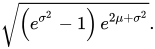
In the case of a parametric family of distributions, the standard deviation can be expressed in terms of the parameters. For example, in the case of the log-normal distribution with parameters μ and σ2, the standard deviation is
Estimation[edit]
One can find the standard deviation of an entire population in cases (such as standardized testing) where every member of a population is sampled. In cases where that cannot be done, the standard deviation σ is estimated by examining a random sample taken from the population and computing a statistic of the sample, which is used as an estimate of the population standard deviation. Such a statistic is called an estimator, and the estimator (or the value of the estimator, namely the estimate) is called a sample standard deviation, and is denoted by s (possibly with modifiers).
Unlike in the case of estimating the population mean, for which the sample mean is a simple estimator with many desirable properties (unbiased, efficient, maximum likelihood), there is no single estimator for the standard deviation with all these properties, and unbiased estimation of standard deviation is a very technically involved problem. Most often, the standard deviation is estimated using the corrected sample standard deviation (using N − 1), defined below, and this is often referred to as the «sample standard deviation», without qualifiers. However, other estimators are better in other respects: the uncorrected estimator (using N) yields lower mean squared error, while using N − 1.5 (for the normal distribution) almost completely eliminates bias.
Uncorrected sample standard deviation[edit]
The formula for the population standard deviation (of a finite population) can be applied to the sample, using the size of the sample as the size of the population (though the actual population size from which the sample is drawn may be much larger). This estimator, denoted by sN, is known as the uncorrected sample standard deviation, or sometimes the standard deviation of the sample (considered as the entire population), and is defined as follows:[6]
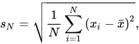
where  are the observed values of the sample items, and
  is the mean value of these observations, while the denominator N stands for the size of the sample: this is the square root of the sample variance, which is the average of the squared deviations about the sample mean.
This is a consistent estimator (it converges in probability to the population value as the number of samples goes to infinity), and is the maximum-likelihood estimate when the population is normally distributed.[7] However, this is a biased estimator, as the estimates are generally too low. The bias decreases as sample size grows, dropping off as 1/N, and thus is most significant for small or moderate sample sizes; for  the bias is below 1%. Thus for very large sample sizes, the uncorrected sample standard deviation is generally acceptable. This estimator also has a uniformly smaller mean squared error than the corrected sample standard deviation.
Corrected sample standard deviation[edit]
If the biased sample variance (the second central moment of the sample, which is a downward-biased estimate of the population variance) is used to compute an estimate of the population’s standard deviation, the result is
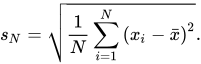
Here taking the square root introduces further downward bias, by Jensen’s inequality, due to the square root’s being a concave function. The bias in the variance is easily corrected, but the bias from the square root is more difficult to correct, and depends on the distribution in question.
An unbiased estimator for the variance is given by applying Bessel’s correction, using N − 1 instead of N to yield the unbiased sample variance, denoted s2:
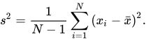
This estimator is unbiased if the variance exists and the sample values are drawn independently with replacement. N − 1 corresponds to the number of degrees of freedom in the vector of deviations from the mean, 
Taking square roots reintroduces bias (because the square root is a nonlinear function which does not commute with the expectation, i.e. often ![{displaystyle E[{sqrt {X}}]neq {sqrt {E[X]}}}](https://wikimedia.org/api/rest_v1/media/math/render/svg/79fa5d2ba8891a41598ddeadc10ba844a20cdfa0) ), yielding the corrected sample standard deviation, denoted by s:
), yielding the corrected sample standard deviation, denoted by s:
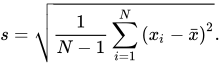
As explained above, while s2 is an unbiased estimator for the population variance, s is still a biased estimator for the population standard deviation, though markedly less biased than the uncorrected sample standard deviation. This estimator is commonly used and generally known simply as the «sample standard deviation». The bias may still be large for small samples (N less than 10). As sample size increases, the amount of bias decreases. We obtain more information and the difference between  and
and  becomes smaller.
Unbiased sample standard deviation[edit]
For unbiased estimation of standard deviation, there is no formula that works across all distributions, unlike for mean and variance. Instead, s is used as a basis, and is scaled by a correction factor to produce an unbiased estimate. For the normal distribution, an unbiased estimator is given by s/c4, where the correction factor (which depends on N) is given in terms of the Gamma function, and equals:
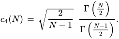
This arises because the sampling distribution of the sample standard deviation follows a (scaled) chi distribution, and the correction factor is the mean of the chi distribution.
An approximation can be given by replacing N − 1 with N − 1.5, yielding:
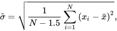
The error in this approximation decays quadratically (as 1/N2), and it is suited for all but the smallest samples or highest precision: for N = 3 the bias is equal to 1.3%, and for N = 9 the bias is already less than 0.1%.
A more accurate approximation is to replace  above with
  .[8]
.[8]
For other distributions, the correct formula depends on the distribution, but a rule of thumb is to use the further refinement of the approximation:
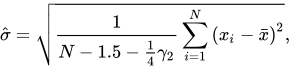
where γ2 denotes the population excess kurtosis. The excess kurtosis may be either known beforehand for certain distributions, or estimated from the data.[9]
Confidence interval of a sampled standard deviation[edit]
The standard deviation we obtain by sampling a distribution is itself not absolutely accurate, both for mathematical reasons (explained here by the confidence interval) and for practical reasons of measurement (measurement error). The mathematical effect can be described by the confidence interval or CI.
To show how a larger sample will make the confidence interval narrower, consider the following examples:
A small population of N = 2 has only 1 degree of freedom for estimating the standard deviation. The result is that a 95% CI of the SD runs from 0.45 × SD to 31.9 × SD; the factors here are as follows:

where  is the p-th quantile of the chi-square distribution with k degrees of freedom, and
  is the confidence level. This is equivalent to the following:
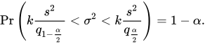
With k = 1,  and
and  . The reciprocals of the square roots of these two numbers give us the factors 0.45 and 31.9 given above.
A larger population of N = 10 has 9 degrees of freedom for estimating the standard deviation. The same computations as above give us in this case a 95% CI running from 0.69 × SD to 1.83 × SD. So even with a sample population of 10, the actual SD can still be almost a factor 2 higher than the sampled SD. For a sample population N=100, this is down to 0.88 × SD to 1.16 × SD. To be more certain that the sampled SD is close to the actual SD we need to sample a large number of points.
These same formulae can be used to obtain confidence intervals on the variance of residuals from a least squares fit under standard normal theory, where k is now the number of degrees of freedom for error.
Bounds on standard deviation[edit]
For a set of N > 4 data spanning a range of values R, an upper bound on the standard deviation s is given by s = 0.6R.[10]
An estimate of the standard deviation for N > 100 data taken to be approximately normal follows from the heuristic that 95% of the area under the normal curve lies roughly two standard deviations to either side of the mean, so that, with 95% probability the total range of values R represents four standard deviations so that s ≈ R/4. This so-called range rule is useful in sample size estimation, as the range of possible values is easier to estimate than the standard deviation. Other divisors K(N) of the range such that s ≈ R/K(N) are available for other values of N and for non-normal distributions.[11]
Identities and mathematical properties[edit]
The standard deviation is invariant under changes in location, and scales directly with the scale of the random variable. Thus, for a constant c and random variables X and Y:
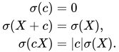
The standard deviation of the sum of two random variables can be related to their individual standard deviations and the covariance between them:

where  and
and  stand for variance and covariance, respectively.
The calculation of the sum of squared deviations can be related to moments calculated directly from the data. In the following formula, the letter E is interpreted to mean expected value, i.e., mean.
![{displaystyle sigma (X)={sqrt {operatorname {E} left[(X-operatorname {E} [X])^{2}right]}}={sqrt {operatorname {E} left[X^{2}right]-(operatorname {E} [X])^{2}}}.}](https://wikimedia.org/api/rest_v1/media/math/render/svg/d3ab12089bd2027790ef060ff7cc2ec05ae2021f)
The sample standard deviation can be computed as:
![{displaystyle s(X)={sqrt {frac {N}{N-1}}}{sqrt {operatorname {E} left[(X-operatorname {E} [X])^{2}right]}}.}](https://wikimedia.org/api/rest_v1/media/math/render/svg/702e9da21c721697e6e81932bf8b7443028f7d6d)
For a finite population with equal probabilities at all points, we have

which means that the standard deviation is equal to the square root of the difference between the average of the squares of the values and the square of the average value.
See computational formula for the variance for proof, and for an analogous result for the sample standard deviation.
Interpretation and application[edit]

Example of samples from two populations with the same mean but different standard deviations. Red population has mean 100 and SD 10; blue population has mean 100 and SD 50.
A large standard deviation indicates that the data points can spread far from the mean and a small standard deviation indicates that they are clustered closely around the mean.
For example, each of the three populations {0, 0, 14, 14}, {0, 6, 8, 14} and {6, 6, 8, 8} has a mean of 7. Their standard deviations are 7, 5, and 1, respectively. The third population has a much smaller standard deviation than the other two because its values are all close to 7. These standard deviations have the same units as the data points themselves. If, for instance, the data set {0, 6, 8, 14} represents the ages of a population of four siblings in years, the standard deviation is 5 years. As another example, the population {1000, 1006, 1008, 1014} may represent the distances traveled by four athletes, measured in meters. It has a mean of 1007 meters, and a standard deviation of 5 meters.
Standard deviation may serve as a measure of uncertainty. In physical science, for example, the reported standard deviation of a group of repeated measurements gives the precision of those measurements. When deciding whether measurements agree with a theoretical prediction, the standard deviation of those measurements is of crucial importance: if the mean of the measurements is too far away from the prediction (with the distance measured in standard deviations), then the theory being tested probably needs to be revised. This makes sense since they fall outside the range of values that could reasonably be expected to occur, if the prediction were correct and the standard deviation appropriately quantified. See prediction interval.
While the standard deviation does measure how far typical values tend to be from the mean, other measures are available. An example is the mean absolute deviation, which might be considered a more direct measure of average distance, compared to the root mean square distance inherent in the standard deviation.
Application examples[edit]
The practical value of understanding the standard deviation of a set of values is in appreciating how much variation there is from the average (mean).
Experiment, industrial and hypothesis testing[edit]
Standard deviation is often used to compare real-world data against a model to test the model.
For example, in industrial applications the weight of products coming off a production line may need to comply with a legally required value. By weighing some fraction of the products an average weight can be found, which will always be slightly different from the long-term average. By using standard deviations, a minimum and maximum value can be calculated that the averaged weight will be within some very high percentage of the time (99.9% or more). If it falls outside the range then the production process may need to be corrected. Statistical tests such as these are particularly important when the testing is relatively expensive. For example, if the product needs to be opened and drained and weighed, or if the product was otherwise used up by the test.
In experimental science, a theoretical model of reality is used. Particle physics conventionally uses a standard of «5 sigma» for the declaration of a discovery. A five-sigma level translates to one chance in 3.5 million that a random fluctuation would yield the result. This level of certainty was required in order to assert that a particle consistent with the Higgs boson had been discovered in two independent experiments at CERN,[12] also leading to the declaration of the first observation of gravitational waves.[13]
Weather[edit]
As a simple example, consider the average daily maximum temperatures for two cities, one inland and one on the coast. It is helpful to understand that the range of daily maximum temperatures for cities near the coast is smaller than for cities inland. Thus, while these two cities may each have the same average maximum temperature, the standard deviation of the daily maximum temperature for the coastal city will be less than that of the inland city as, on any particular day, the actual maximum temperature is more likely to be farther from the average maximum temperature for the inland city than for the coastal one.
Finance[edit]
In finance, standard deviation is often used as a measure of the risk associated with price-fluctuations of a given asset (stocks, bonds, property, etc.), or the risk of a portfolio of assets[14] (actively managed mutual funds, index mutual funds, or ETFs). Risk is an important factor in determining how to efficiently manage a portfolio of investments because it determines the variation in returns on the asset and/or portfolio and gives investors a mathematical basis for investment decisions (known as mean-variance optimization). The fundamental concept of risk is that as it increases, the expected return on an investment should increase as well, an increase known as the risk premium. In other words, investors should expect a higher return on an investment when that investment carries a higher level of risk or uncertainty. When evaluating investments, investors should estimate both the expected return and the uncertainty of future returns. Standard deviation provides a quantified estimate of the uncertainty of future returns.
For example, assume an investor had to choose between two stocks. Stock A over the past 20 years had an average return of 10 percent, with a standard deviation of 20 percentage points (pp) and Stock B, over the same period, had average returns of 12 percent but a higher standard deviation of 30 pp. On the basis of risk and return, an investor may decide that Stock A is the safer choice, because Stock B’s additional two percentage points of return is not worth the additional 10 pp standard deviation (greater risk or uncertainty of the expected return). Stock B is likely to fall short of the initial investment (but also to exceed the initial investment) more often than Stock A under the same circumstances, and is estimated to return only two percent more on average. In this example, Stock A is expected to earn about 10 percent, plus or minus 20 pp (a range of 30 percent to −10 percent), about two-thirds of the future year returns. When considering more extreme possible returns or outcomes in future, an investor should expect results of as much as 10 percent plus or minus 60 pp, or a range from 70 percent to −50 percent, which includes outcomes for three standard deviations from the average return (about 99.7 percent of probable returns).
Calculating the average (or arithmetic mean) of the return of a security over a given period will generate the expected return of the asset. For each period, subtracting the expected return from the actual return results in the difference from the mean. Squaring the difference in each period and taking the average gives the overall variance of the return of the asset. The larger the variance, the greater risk the security carries. Finding the square root of this variance will give the standard deviation of the investment tool in question.
Population standard deviation is used to set the width of Bollinger Bands, a technical analysis tool. For example, the upper Bollinger Band is given as  The most commonly used value for n is 2; there is about a five percent chance of going outside, assuming a normal distribution of returns.
Financial time series are known to be non-stationary series, whereas the statistical calculations above, such as standard deviation, apply only to stationary series. To apply the above statistical tools to non-stationary series, the series first must be transformed to a stationary series, enabling use of statistical tools that now have a valid basis from which to work.
Geometric interpretation[edit]
To gain some geometric insights and clarification, we will start with a population of three values, x1, x2, x3. This defines a point P = (x1, x2, x3) in R3. Consider the line L = {(r, r, r) : r ∈ R}. This is the «main diagonal» going through the origin. If our three given values were all equal, then the standard deviation would be zero and P would lie on L. So it is not unreasonable to assume that the standard deviation is related to the distance of P to L. That is indeed the case. To move orthogonally from L to the point P, one begins at the point:
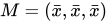
whose coordinates are the mean of the values we started out with.
A little algebra shows that the distance between P and M (which is the same as the orthogonal distance between P and the line L) 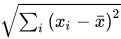 is equal to the standard deviation of the vector (x1, x2, x3), multiplied by the square root of the number of dimensions of the vector (3 in this case).
Chebyshev’s inequality[edit]
An observation is rarely more than a few standard deviations away from the mean. Chebyshev’s inequality ensures that, for all distributions for which the standard deviation is defined, the amount of data within a number of standard deviations of the mean is at least as much as given in the following table.
| Distance from mean | Minimum population |
|---|---|
 |
50% |
| 2σ | 75% |
| 3σ | 89% |
| 4σ | 94% |
| 5σ | 96% |
| 6σ | 97% |
 |
 [15] [15]
|
 |

|
Rules for normally distributed data[edit]
Dark blue is one standard deviation on either side of the mean. For the normal distribution, this accounts for 68.27 percent of the set; while two standard deviations from the mean (medium and dark blue) account for 95.45 percent; three standard deviations (light, medium, and dark blue) account for 99.73 percent; and four standard deviations account for 99.994 percent. The two points of the curve that are one standard deviation from the mean are also the inflection points.
The central limit theorem states that the distribution of an average of many independent, identically distributed random variables tends toward the famous bell-shaped normal distribution with a probability density function of
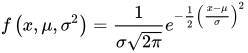
where μ is the expected value of the random variables, σ equals their distribution’s standard deviation divided by n1/2, and n is the number of random variables. The standard deviation therefore is simply a scaling variable that adjusts how broad the curve will be, though it also appears in the normalizing constant.
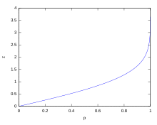
If a data distribution is approximately normal, then the proportion of data values within z standard deviations of the mean is defined by:
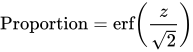
where  is the error function. The proportion that is less than or equal to a number, x, is given by the cumulative distribution function:
![{displaystyle {text{Proportion}}leq x={frac {1}{2}}left[1+operatorname {erf} left({frac {x-mu }{sigma {sqrt {2}}}}right)right]={frac {1}{2}}left[1+operatorname {erf} left({frac {z}{sqrt {2}}}right)right]}](data:image/svg+xml,%3Csvg%20xmlns='http://www.w3.org/2000/svg'%20viewBox='0%200%200%200'%3E%3C/svg%3E) .[16]
.[16]
![{displaystyle {text{Proportion}}leq x={frac {1}{2}}left[1+operatorname {erf} left({frac {x-mu }{sigma {sqrt {2}}}}right)right]={frac {1}{2}}left[1+operatorname {erf} left({frac {z}{sqrt {2}}}right)right]}](https://wikimedia.org/api/rest_v1/media/math/render/svg/3907d1b0502235fa3fd00f261b290406a02e7b21)
If a data distribution is approximately normal then about 68 percent of the data values are within one standard deviation of the mean (mathematically, μ ± σ, where μ is the arithmetic mean), about 95 percent are within two standard deviations (μ ± 2σ), and about 99.7 percent lie within three standard deviations (μ ± 3σ). This is known as the 68–95–99.7 rule, or the empirical rule.
For various values of z, the percentage of values expected to lie in and outside the symmetric interval, CI = (−zσ, zσ), are as follows:
| Confidence interval |
Proportion within | Proportion without | |
|---|---|---|---|
| Percentage | Percentage | Fraction | |
| 0.318639σ | 25% | 75% | 3 / 4 |
| 0.674490σ | 50% | 50% | 1 / 2 |
| 0.977925σ | 66.6667% | 33.3333% | 1 / 3 |
| 0.994458σ | 68% | 32% | 1 / 3.125 |
| 1σ | 68.2689492% | 31.7310508% | 1 / 3.1514872 |
| 1.281552σ | 80% | 20% | 1 / 5 |
| 1.644854σ | 90% | 10% | 1 / 10 |
| 1.959964σ | 95% | 5% | 1 / 20 |
| 2σ | 95.4499736% | 4.5500264% | 1 / 21.977895 |
| 2.575829σ | 99% | 1% | 1 / 100 |
| 3σ | 99.7300204% | 0.2699796% | 1 / 370.398 |
| 3.290527σ | 99.9% | 0.1% | 1 / 1000 |
| 3.890592σ | 99.99% | 0.01% | 1 / 10000 |
| 4σ | 99.993666% | 0.006334% | 1 / 15787 |
| 4.417173σ | 99.999% | 0.001% | 1 / 100000 |
| 4.5σ | 99.9993204653751% | 0.0006795346249% | 1 / 147159.5358 6.8 / 1000000 |
| 4.891638σ | 99.9999% | 0.0001% | 1 / 1000000 |
| 5σ | 99.9999426697% | 0.0000573303% | 1 / 1744278 |
| 5.326724σ | 99.99999% | 0.00001% | 1 / 10000000 |
| 5.730729σ | 99.999999% | 0.000001% | 1 / 100000000 |
| 6σ | 99.9999998027% | 0.0000001973% | 1 / 506797346 |
| 6.109410σ | 99.9999999% | 0.0000001% | 1 / 1000000000 |
| 6.466951σ | 99.99999999% | 0.00000001% | 1 / 10000000000 |
| 6.806502σ | 99.999999999% | 0.000000001% | 1 / 100000000000 |
| 7σ | 99.9999999997440% | 0.000000000256% | 1 / 390682215445 |
Relationship between standard deviation and mean[edit]
The mean and the standard deviation of a set of data are descriptive statistics usually reported together. In a certain sense, the standard deviation is a «natural» measure of statistical dispersion if the center of the data is measured about the mean. This is because the standard deviation from the mean is smaller than from any other point. The precise statement is the following: suppose x1, …, xn are real numbers and define the function:
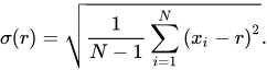
Using calculus or by completing the square, it is possible to show that σ(r) has a unique minimum at the mean:

Variability can also be measured by the coefficient of variation, which is the ratio of the standard deviation to the mean. It is a dimensionless number.
Standard deviation of the mean[edit]
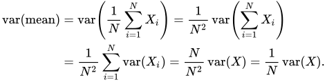
Often, we want some information about the precision of the mean we obtained. We can obtain this by determining the standard deviation of the sampled mean. Assuming statistical independence of the values in the sample, the standard deviation of the mean is related to the standard deviation of the distribution by:
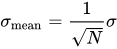
where N is the number of observations in the sample used to estimate the mean. This can easily be proven with (see basic properties of the variance):

(Statistical independence is assumed.)

hence
Resulting in:
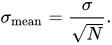
In order to estimate the standard deviation of the mean  it is necessary to know the standard deviation of the entire population
  beforehand. However, in most applications this parameter is unknown. For example, if a series of 10 measurements of a previously unknown quantity is performed in a laboratory, it is possible to calculate the resulting sample mean and sample standard deviation, but it is impossible to calculate the standard deviation of the mean. However, one can estimate the standard deviation of the entire population from the sample, and thus obtain an estimate for the standard error of the mean.
Rapid calculation methods[edit]
The following two formulas can represent a running (repeatedly updated) standard deviation. A set of two power sums s1 and s2 are computed over a set of N values of x, denoted as x1, …, xN:

Given the results of these running summations, the values N, s1, s2 can be used at any time to compute the current value of the running standard deviation:
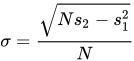
Where N, as mentioned above, is the size of the set of values (or can also be regarded as s0).
Similarly for sample standard deviation,
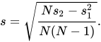
In a computer implementation, as the two sj sums become large, we need to consider round-off error, arithmetic overflow, and arithmetic underflow. The method below calculates the running sums method with reduced rounding errors.[17] This is a «one pass» algorithm for calculating variance of n samples without the need to store prior data during the calculation. Applying this method to a time series will result in successive values of standard deviation corresponding to n data points as n grows larger with each new sample, rather than a constant-width sliding window calculation.
For k = 1, …, n:
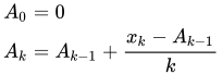
where A is the mean value.

Note:  since
since  or
or 
Sample variance:

Population variance:

Weighted calculation[edit]
When the values xi are weighted with unequal weights wi, the power sums s0, s1, s2 are each computed as:
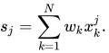
And the standard deviation equations remain unchanged. s0 is now the sum of the weights and not the number of samples N.
The incremental method with reduced rounding errors can also be applied, with some additional complexity.
A running sum of weights must be computed for each k from 1 to n:
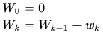
and places where 1/n is used above must be replaced by wi/Wn:
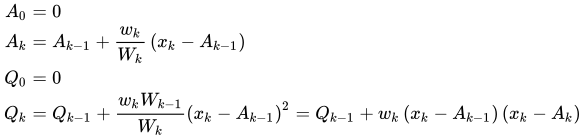
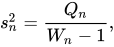
In the final division,

and
or

where n is the total number of elements, and n’ is the number of elements with non-zero weights.
The above formulas become equal to the simpler formulas given above if weights are taken as equal to one.
History[edit]
The term standard deviation was first used in writing by Karl Pearson in 1894, following his use of it in lectures.[18][19] This was as a replacement for earlier alternative names for the same idea: for example, Gauss used mean error.[20]
Higher dimensions[edit]
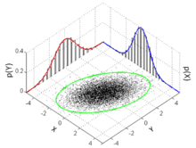
The standard deviation ellipse (green) of a two-dimensional normal distribution
In two dimensions, the standard deviation can be illustrated with the standard deviation ellipse (see Multivariate normal distribution § Geometric interpretation).
See also[edit]
- 68–95–99.7 rule
- Accuracy and precision
- Chebyshev’s inequality An inequality on location and scale parameters
- Coefficient of variation
- Cumulant
- Deviation (statistics)
- Distance correlation Distance standard deviation
- Error bar
- Geometric standard deviation
- Mahalanobis distance generalizing number of standard deviations to the mean
- Mean absolute error
- Pooled variance
- Propagation of uncertainty
- Percentile
- Raw data
- Robust standard deviation
- Root mean square
- Sample size
- Samuelson’s inequality
- Six Sigma
- Standard error
- Standard score
- Yamartino method for calculating standard deviation of wind direction
References[edit]
- ^ Bland, J.M.; Altman, D.G. (1996). «Statistics notes: measurement error». BMJ. 312 (7047): 1654. doi:10.1136/bmj.312.7047.1654. PMC 2351401. PMID 8664723.
- ^ Gauss, Carl Friedrich (1816). «Bestimmung der Genauigkeit der Beobachtungen». Zeitschrift für Astronomie und Verwandte Wissenschaften. 1: 187–197.
- ^ Walker, Helen (1931). Studies in the History of the Statistical Method. Baltimore, MD: Williams & Wilkins Co. pp. 24–25.
- ^ Weisstein, Eric W. «Bessel’s Correction». MathWorld.
- ^ «Standard Deviation Formulas». www.mathsisfun.com. Retrieved 21 August 2020.
- ^ Weisstein, Eric W. «Standard Deviation». mathworld.wolfram.com. Retrieved 21 August 2020.
- ^ «Consistent estimator». www.statlect.com. Retrieved 10 October 2022.
- ^ Gurland, John; Tripathi, Ram C. (1971), «A Simple Approximation for Unbiased Estimation of the Standard Deviation», The American Statistician, 25 (4): 30–32, doi:10.2307/2682923, JSTOR 2682923
- ^ «Standard Deviation Calculator». PureCalculators. 11 July 2021. Retrieved 14 September 2021.
- ^ Shiffler, Ronald E.; Harsha, Phillip D. (1980). «Upper and Lower Bounds for the Sample Standard Deviation». Teaching Statistics. 2 (3): 84–86. doi:10.1111/j.1467-9639.1980.tb00398.x.
- ^ Browne, Richard H. (2001). «Using the Sample Range as a Basis for Calculating Sample Size in Power Calculations». The American Statistician. 55 (4): 293–298. doi:10.1198/000313001753272420. JSTOR 2685690. S2CID 122328846.
- ^ «CERN experiments observe particle consistent with long-sought Higgs boson | CERN press office». Press.web.cern.ch. 4 July 2012. Archived from the original on 25 March 2016. Retrieved 30 May 2015.
- ^ LIGO Scientific Collaboration, Virgo Collaboration (2016), «Observation of Gravitational Waves from a Binary Black Hole Merger», Physical Review Letters, 116 (6): 061102, arXiv:1602.03837, Bibcode:2016PhRvL.116f1102A, doi:10.1103/PhysRevLett.116.061102, PMID 26918975, S2CID 124959784
- ^ «What is Standard Deviation». Pristine. Retrieved 29 October 2011.
- ^ Ghahramani, Saeed (2000). Fundamentals of Probability (2nd ed.). New Jersey: Prentice Hall. p. 438. ISBN 9780130113290.
- ^ Eric W. Weisstein. «Distribution Function». MathWorld—A Wolfram Web Resource. Retrieved 30 September 2014.
- ^ Welford, BP (August 1962). «Note on a Method for Calculating Corrected Sums of Squares and Products». Technometrics. 4 (3): 419–420. CiteSeerX 10.1.1.302.7503. doi:10.1080/00401706.1962.10490022.
- ^ Dodge, Yadolah (2003). The Oxford Dictionary of Statistical Terms. Oxford University Press. ISBN 978-0-19-920613-1.
- ^ Pearson, Karl (1894). «On the dissection of asymmetrical frequency curves». Philosophical Transactions of the Royal Society A. 185: 71–110. Bibcode:1894RSPTA.185…71P. doi:10.1098/rsta.1894.0003.
- ^ Miller, Jeff. «Earliest Known Uses of Some of the Words of Mathematics».
External links[edit]
- «Quadratic deviation», Encyclopedia of Mathematics, EMS Press, 2001 [1994]
- «Standard Deviation Calculator»
Cumulative probability of a normal distribution with expected value 0 and standard deviation 1
In statistics, the standard deviation is a measure of the amount of variation or dispersion of a set of values.[1] A low standard deviation indicates that the values tend to be close to the mean (also called the expected value) of the set, while a high standard deviation indicates that the values are spread out over a wider range.
Standard deviation may be abbreviated SD, and is most commonly represented in mathematical texts and equations by the lower case Greek letter σ (sigma), for the population standard deviation, or the Latin letter s, for the sample standard deviation.
The standard deviation of a random variable, sample, statistical population, data set, or probability distribution is the square root of its variance. It is algebraically simpler, though in practice less robust, than the average absolute deviation.[2][3] A useful property of the standard deviation is that, unlike the variance, it is expressed in the same unit as the data.
The standard deviation of a population or sample and the standard error of a statistic (e.g., of the sample mean) are quite different, but related. The sample mean’s standard error is the standard deviation of the set of means that would be found by drawing an infinite number of repeated samples from the population and computing a mean for each sample. The mean’s standard error turns out to equal the population standard deviation divided by the square root of the sample size, and is estimated by using the sample standard deviation divided by the square root of the sample size. For example, a poll’s standard error (what is reported as the margin of error of the poll), is the expected standard deviation of the estimated mean if the same poll were to be conducted multiple times. Thus, the standard error estimates the standard deviation of an estimate, which itself measures how much the estimate depends on the particular sample that was taken from the population.
In science, it is common to report both the standard deviation of the data (as a summary statistic) and the standard error of the estimate (as a measure of potential error in the findings). By convention, only effects more than two standard errors away from a null expectation are considered «statistically significant», a safeguard against spurious conclusion that is really due to random sampling error.
When only a sample of data from a population is available, the term standard deviation of the sample or sample standard deviation can refer to either the above-mentioned quantity as applied to those data, or to a modified quantity that is an unbiased estimate of the population standard deviation (the standard deviation of the entire population).
Basic examples[edit]
Population standard deviation of grades of eight students[edit]
Suppose that the entire population of interest is eight students in a particular class. For a finite set of numbers, the population standard deviation is found by taking the square root of the average of the squared deviations of the values subtracted from their average value. The marks of a class of eight students (that is, a statistical population) are the following eight values:
These eight data points have the mean (average) of 5:
First, calculate the deviations of each data point from the mean, and square the result of each:
The variance is the mean of these values:
and the population standard deviation is equal to the square root of the variance:
This formula is valid only if the eight values with which we began form the complete population. If the values instead were a random sample drawn from some large parent population (for example, they were 8 students randomly and independently chosen from a class of 2 million), then one divides by 7 (which is n − 1) instead of 8 (which is n) in the denominator of the last formula, and the result is In that case, the result of the original formula would be called the sample standard deviation and denoted by s instead of Dividing by n − 1 rather than by n gives an unbiased estimate of the variance of the larger parent population. This is known as Bessel’s correction.[4][5] Roughly, the reason for it is that the formula for the sample variance relies on computing differences of observations from the sample mean, and the sample mean itself was constructed to be as close as possible to the observations, so just dividing by n would underestimate the variability.
Standard deviation of average height for adult men[edit]
If the population of interest is approximately normally distributed, the standard deviation provides information on the proportion of observations above or below certain values. For example, the average height for adult men in the United States is about 70 inches, with a standard deviation of around 3 inches. This means that most men (about 68%, assuming a normal distribution) have a height within 3 inches of the mean (67–73 inches) – one standard deviation – and almost all men (about 95%) have a height within 6 inches of the mean (64–76 inches) – two standard deviations. If the standard deviation were zero, then all men would be exactly 70 inches tall. If the standard deviation were 20 inches, then men would have much more variable heights, with a typical range of about 50–90 inches. Three standard deviations account for 99.73% of the sample population being studied, assuming the distribution is normal or bell-shaped (see the 68–95–99.7 rule, or the empirical rule, for more information).
Definition of population values[edit]
Let μ be the expected value (the average) of random variable X with density f(x):
The standard deviation σ of X is defined as
which can be shown to equal
Using words, the standard deviation is the square root of the variance of X.
The standard deviation of a probability distribution is the same as that of a random variable having that distribution.
Not all random variables have a standard deviation. If the distribution has fat tails going out to infinity, the standard deviation might not exist, because the integral might not converge. The normal distribution has tails going out to infinity, but its mean and standard deviation do exist, because the tails diminish quickly enough. The Pareto distribution with parameter has a mean, but not a standard deviation (loosely speaking, the standard deviation is infinite). The Cauchy distribution has neither a mean nor a standard deviation.
Discrete random variable[edit]
In the case where X takes random values from a finite data set x1, x2, …, xN, with each value having the same probability, the standard deviation is
or, by using summation notation,
If, instead of having equal probabilities, the values have different probabilities, let x1 have probability p1, x2 have probability p2, …, xN have probability pN. In this case, the standard deviation will be
Continuous random variable[edit]
The standard deviation of a continuous real-valued random variable X with probability density function p(x) is
and where the integrals are definite integrals taken for x ranging over the set of possible values of the random variable X.
In the case of a parametric family of distributions, the standard deviation can be expressed in terms of the parameters. For example, in the case of the log-normal distribution with parameters μ and σ2, the standard deviation is
Estimation[edit]
One can find the standard deviation of an entire population in cases (such as standardized testing) where every member of a population is sampled. In cases where that cannot be done, the standard deviation σ is estimated by examining a random sample taken from the population and computing a statistic of the sample, which is used as an estimate of the population standard deviation. Such a statistic is called an estimator, and the estimator (or the value of the estimator, namely the estimate) is called a sample standard deviation, and is denoted by s (possibly with modifiers).
Unlike in the case of estimating the population mean, for which the sample mean is a simple estimator with many desirable properties (unbiased, efficient, maximum likelihood), there is no single estimator for the standard deviation with all these properties, and unbiased estimation of standard deviation is a very technically involved problem. Most often, the standard deviation is estimated using the corrected sample standard deviation (using N − 1), defined below, and this is often referred to as the «sample standard deviation», without qualifiers. However, other estimators are better in other respects: the uncorrected estimator (using N) yields lower mean squared error, while using N − 1.5 (for the normal distribution) almost completely eliminates bias.
Uncorrected sample standard deviation[edit]
The formula for the population standard deviation (of a finite population) can be applied to the sample, using the size of the sample as the size of the population (though the actual population size from which the sample is drawn may be much larger). This estimator, denoted by sN, is known as the uncorrected sample standard deviation, or sometimes the standard deviation of the sample (considered as the entire population), and is defined as follows:[6]
where are the observed values of the sample items, and is the mean value of these observations, while the denominator N stands for the size of the sample: this is the square root of the sample variance, which is the average of the squared deviations about the sample mean.
This is a consistent estimator (it converges in probability to the population value as the number of samples goes to infinity), and is the maximum-likelihood estimate when the population is normally distributed.[7] However, this is a biased estimator, as the estimates are generally too low. The bias decreases as sample size grows, dropping off as 1/N, and thus is most significant for small or moderate sample sizes; for the bias is below 1%. Thus for very large sample sizes, the uncorrected sample standard deviation is generally acceptable. This estimator also has a uniformly smaller mean squared error than the corrected sample standard deviation.
Corrected sample standard deviation[edit]
If the biased sample variance (the second central moment of the sample, which is a downward-biased estimate of the population variance) is used to compute an estimate of the population’s standard deviation, the result is
Here taking the square root introduces further downward bias, by Jensen’s inequality, due to the square root’s being a concave function. The bias in the variance is easily corrected, but the bias from the square root is more difficult to correct, and depends on the distribution in question.
An unbiased estimator for the variance is given by applying Bessel’s correction, using N − 1 instead of N to yield the unbiased sample variance, denoted s2:
This estimator is unbiased if the variance exists and the sample values are drawn independently with replacement. N − 1 corresponds to the number of degrees of freedom in the vector of deviations from the mean,
Taking square roots reintroduces bias (because the square root is a nonlinear function which does not commute with the expectation, i.e. often ), yielding the corrected sample standard deviation, denoted by s:
As explained above, while s2 is an unbiased estimator for the population variance, s is still a biased estimator for the population standard deviation, though markedly less biased than the uncorrected sample standard deviation. This estimator is commonly used and generally known simply as the «sample standard deviation». The bias may still be large for small samples (N less than 10). As sample size increases, the amount of bias decreases. We obtain more information and the difference between and becomes smaller.
Unbiased sample standard deviation[edit]
For unbiased estimation of standard deviation, there is no formula that works across all distributions, unlike for mean and variance. Instead, s is used as a basis, and is scaled by a correction factor to produce an unbiased estimate. For the normal distribution, an unbiased estimator is given by s/c4, where the correction factor (which depends on N) is given in terms of the Gamma function, and equals:
This arises because the sampling distribution of the sample standard deviation follows a (scaled) chi distribution, and the correction factor is the mean of the chi distribution.
An approximation can be given by replacing N − 1 with N − 1.5, yielding:
The error in this approximation decays quadratically (as 1/N2), and it is suited for all but the smallest samples or highest precision: for N = 3 the bias is equal to 1.3%, and for N = 9 the bias is already less than 0.1%.
A more accurate approximation is to replace above with .[8]
For other distributions, the correct formula depends on the distribution, but a rule of thumb is to use the further refinement of the approximation:
where γ2 denotes the population excess kurtosis. The excess kurtosis may be either known beforehand for certain distributions, or estimated from the data.[9]
Confidence interval of a sampled standard deviation[edit]
The standard deviation we obtain by sampling a distribution is itself not absolutely accurate, both for mathematical reasons (explained here by the confidence interval) and for practical reasons of measurement (measurement error). The mathematical effect can be described by the confidence interval or CI.
To show how a larger sample will make the confidence interval narrower, consider the following examples:
A small population of N = 2 has only 1 degree of freedom for estimating the standard deviation. The result is that a 95% CI of the SD runs from 0.45 × SD to 31.9 × SD; the factors here are as follows:
where is the p-th quantile of the chi-square distribution with k degrees of freedom, and is the confidence level. This is equivalent to the following:
With k = 1, and . The reciprocals of the square roots of these two numbers give us the factors 0.45 and 31.9 given above.
A larger population of N = 10 has 9 degrees of freedom for estimating the standard deviation. The same computations as above give us in this case a 95% CI running from 0.69 × SD to 1.83 × SD. So even with a sample population of 10, the actual SD can still be almost a factor 2 higher than the sampled SD. For a sample population N=100, this is down to 0.88 × SD to 1.16 × SD. To be more certain that the sampled SD is close to the actual SD we need to sample a large number of points.
These same formulae can be used to obtain confidence intervals on the variance of residuals from a least squares fit under standard normal theory, where k is now the number of degrees of freedom for error.
Bounds on standard deviation[edit]
For a set of N > 4 data spanning a range of values R, an upper bound on the standard deviation s is given by s = 0.6R.[10]
An estimate of the standard deviation for N > 100 data taken to be approximately normal follows from the heuristic that 95% of the area under the normal curve lies roughly two standard deviations to either side of the mean, so that, with 95% probability the total range of values R represents four standard deviations so that s ≈ R/4. This so-called range rule is useful in sample size estimation, as the range of possible values is easier to estimate than the standard deviation. Other divisors K(N) of the range such that s ≈ R/K(N) are available for other values of N and for non-normal distributions.[11]
Identities and mathematical properties[edit]
The standard deviation is invariant under changes in location, and scales directly with the scale of the random variable. Thus, for a constant c and random variables X and Y:
The standard deviation of the sum of two random variables can be related to their individual standard deviations and the covariance between them:
where and stand for variance and covariance, respectively.
The calculation of the sum of squared deviations can be related to moments calculated directly from the data. In the following formula, the letter E is interpreted to mean expected value, i.e., mean.
The sample standard deviation can be computed as:
For a finite population with equal probabilities at all points, we have
which means that the standard deviation is equal to the square root of the difference between the average of the squares of the values and the square of the average value.
See computational formula for the variance for proof, and for an analogous result for the sample standard deviation.
Interpretation and application[edit]
Example of samples from two populations with the same mean but different standard deviations. Red population has mean 100 and SD 10; blue population has mean 100 and SD 50.
A large standard deviation indicates that the data points can spread far from the mean and a small standard deviation indicates that they are clustered closely around the mean.
For example, each of the three populations {0, 0, 14, 14}, {0, 6, 8, 14} and {6, 6, 8, 8} has a mean of 7. Their standard deviations are 7, 5, and 1, respectively. The third population has a much smaller standard deviation than the other two because its values are all close to 7. These standard deviations have the same units as the data points themselves. If, for instance, the data set {0, 6, 8, 14} represents the ages of a population of four siblings in years, the standard deviation is 5 years. As another example, the population {1000, 1006, 1008, 1014} may represent the distances traveled by four athletes, measured in meters. It has a mean of 1007 meters, and a standard deviation of 5 meters.
Standard deviation may serve as a measure of uncertainty. In physical science, for example, the reported standard deviation of a group of repeated measurements gives the precision of those measurements. When deciding whether measurements agree with a theoretical prediction, the standard deviation of those measurements is of crucial importance: if the mean of the measurements is too far away from the prediction (with the distance measured in standard deviations), then the theory being tested probably needs to be revised. This makes sense since they fall outside the range of values that could reasonably be expected to occur, if the prediction were correct and the standard deviation appropriately quantified. See prediction interval.
While the standard deviation does measure how far typical values tend to be from the mean, other measures are available. An example is the mean absolute deviation, which might be considered a more direct measure of average distance, compared to the root mean square distance inherent in the standard deviation.
Application examples[edit]
The practical value of understanding the standard deviation of a set of values is in appreciating how much variation there is from the average (mean).
Experiment, industrial and hypothesis testing[edit]
Standard deviation is often used to compare real-world data against a model to test the model.
For example, in industrial applications the weight of products coming off a production line may need to comply with a legally required value. By weighing some fraction of the products an average weight can be found, which will always be slightly different from the long-term average. By using standard deviations, a minimum and maximum value can be calculated that the averaged weight will be within some very high percentage of the time (99.9% or more). If it falls outside the range then the production process may need to be corrected. Statistical tests such as these are particularly important when the testing is relatively expensive. For example, if the product needs to be opened and drained and weighed, or if the product was otherwise used up by the test.
In experimental science, a theoretical model of reality is used. Particle physics conventionally uses a standard of «5 sigma» for the declaration of a discovery. A five-sigma level translates to one chance in 3.5 million that a random fluctuation would yield the result. This level of certainty was required in order to assert that a particle consistent with the Higgs boson had been discovered in two independent experiments at CERN,[12] also leading to the declaration of the first observation of gravitational waves.[13]
Weather[edit]
As a simple example, consider the average daily maximum temperatures for two cities, one inland and one on the coast. It is helpful to understand that the range of daily maximum temperatures for cities near the coast is smaller than for cities inland. Thus, while these two cities may each have the same average maximum temperature, the standard deviation of the daily maximum temperature for the coastal city will be less than that of the inland city as, on any particular day, the actual maximum temperature is more likely to be farther from the average maximum temperature for the inland city than for the coastal one.
Finance[edit]
In finance, standard deviation is often used as a measure of the risk associated with price-fluctuations of a given asset (stocks, bonds, property, etc.), or the risk of a portfolio of assets[14] (actively managed mutual funds, index mutual funds, or ETFs). Risk is an important factor in determining how to efficiently manage a portfolio of investments because it determines the variation in returns on the asset and/or portfolio and gives investors a mathematical basis for investment decisions (known as mean-variance optimization). The fundamental concept of risk is that as it increases, the expected return on an investment should increase as well, an increase known as the risk premium. In other words, investors should expect a higher return on an investment when that investment carries a higher level of risk or uncertainty. When evaluating investments, investors should estimate both the expected return and the uncertainty of future returns. Standard deviation provides a quantified estimate of the uncertainty of future returns.
For example, assume an investor had to choose between two stocks. Stock A over the past 20 years had an average return of 10 percent, with a standard deviation of 20 percentage points (pp) and Stock B, over the same period, had average returns of 12 percent but a higher standard deviation of 30 pp. On the basis of risk and return, an investor may decide that Stock A is the safer choice, because Stock B’s additional two percentage points of return is not worth the additional 10 pp standard deviation (greater risk or uncertainty of the expected return). Stock B is likely to fall short of the initial investment (but also to exceed the initial investment) more often than Stock A under the same circumstances, and is estimated to return only two percent more on average. In this example, Stock A is expected to earn about 10 percent, plus or minus 20 pp (a range of 30 percent to −10 percent), about two-thirds of the future year returns. When considering more extreme possible returns or outcomes in future, an investor should expect results of as much as 10 percent plus or minus 60 pp, or a range from 70 percent to −50 percent, which includes outcomes for three standard deviations from the average return (about 99.7 percent of probable returns).
Calculating the average (or arithmetic mean) of the return of a security over a given period will generate the expected return of the asset. For each period, subtracting the expected return from the actual return results in the difference from the mean. Squaring the difference in each period and taking the average gives the overall variance of the return of the asset. The larger the variance, the greater risk the security carries. Finding the square root of this variance will give the standard deviation of the investment tool in question.
Population standard deviation is used to set the width of Bollinger Bands, a technical analysis tool. For example, the upper Bollinger Band is given as The most commonly used value for n is 2; there is about a five percent chance of going outside, assuming a normal distribution of returns.
Financial time series are known to be non-stationary series, whereas the statistical calculations above, such as standard deviation, apply only to stationary series. To apply the above statistical tools to non-stationary series, the series first must be transformed to a stationary series, enabling use of statistical tools that now have a valid basis from which to work.
Geometric interpretation[edit]
To gain some geometric insights and clarification, we will start with a population of three values, x1, x2, x3. This defines a point P = (x1, x2, x3) in R3. Consider the line L = {(r, r, r) : r ∈ R}. This is the «main diagonal» going through the origin. If our three given values were all equal, then the standard deviation would be zero and P would lie on L. So it is not unreasonable to assume that the standard deviation is related to the distance of P to L. That is indeed the case. To move orthogonally from L to the point P, one begins at the point:
whose coordinates are the mean of the values we started out with.
A little algebra shows that the distance between P and M (which is the same as the orthogonal distance between P and the line L) is equal to the standard deviation of the vector (x1, x2, x3), multiplied by the square root of the number of dimensions of the vector (3 in this case).
Chebyshev’s inequality[edit]
An observation is rarely more than a few standard deviations away from the mean. Chebyshev’s inequality ensures that, for all distributions for which the standard deviation is defined, the amount of data within a number of standard deviations of the mean is at least as much as given in the following table.
| Distance from mean | Minimum population |
|---|---|
|
50% |
| 2σ | 75% |
| 3σ | 89% |
| 4σ | 94% |
| 5σ | 96% |
| 6σ | 97% |
|
[15]
|
|
|
Rules for normally distributed data[edit]
Dark blue is one standard deviation on either side of the mean. For the normal distribution, this accounts for 68.27 percent of the set; while two standard deviations from the mean (medium and dark blue) account for 95.45 percent; three standard deviations (light, medium, and dark blue) account for 99.73 percent; and four standard deviations account for 99.994 percent. The two points of the curve that are one standard deviation from the mean are also the inflection points.
The central limit theorem states that the distribution of an average of many independent, identically distributed random variables tends toward the famous bell-shaped normal distribution with a probability density function of
where μ is the expected value of the random variables, σ equals their distribution’s standard deviation divided by n1/2, and n is the number of random variables. The standard deviation therefore is simply a scaling variable that adjusts how broad the curve will be, though it also appears in the normalizing constant.
If a data distribution is approximately normal, then the proportion of data values within z standard deviations of the mean is defined by:
where is the error function. The proportion that is less than or equal to a number, x, is given by the cumulative distribution function:
- .[16]
If a data distribution is approximately normal then about 68 percent of the data values are within one standard deviation of the mean (mathematically, μ ± σ, where μ is the arithmetic mean), about 95 percent are within two standard deviations (μ ± 2σ), and about 99.7 percent lie within three standard deviations (μ ± 3σ). This is known as the 68–95–99.7 rule, or the empirical rule.
For various values of z, the percentage of values expected to lie in and outside the symmetric interval, CI = (−zσ, zσ), are as follows:
| Confidence interval |
Proportion within | Proportion without | |
|---|---|---|---|
| Percentage | Percentage | Fraction | |
| 0.318639σ | 25% | 75% | 3 / 4 |
| 0.674490σ | 50% | 50% | 1 / 2 |
| 0.977925σ | 66.6667% | 33.3333% | 1 / 3 |
| 0.994458σ | 68% | 32% | 1 / 3.125 |
| 1σ | 68.2689492% | 31.7310508% | 1 / 3.1514872 |
| 1.281552σ | 80% | 20% | 1 / 5 |
| 1.644854σ | 90% | 10% | 1 / 10 |
| 1.959964σ | 95% | 5% | 1 / 20 |
| 2σ | 95.4499736% | 4.5500264% | 1 / 21.977895 |
| 2.575829σ | 99% | 1% | 1 / 100 |
| 3σ | 99.7300204% | 0.2699796% | 1 / 370.398 |
| 3.290527σ | 99.9% | 0.1% | 1 / 1000 |
| 3.890592σ | 99.99% | 0.01% | 1 / 10000 |
| 4σ | 99.993666% | 0.006334% | 1 / 15787 |
| 4.417173σ | 99.999% | 0.001% | 1 / 100000 |
| 4.5σ | 99.9993204653751% | 0.0006795346249% | 1 / 147159.5358 6.8 / 1000000 |
| 4.891638σ | 99.9999% | 0.0001% | 1 / 1000000 |
| 5σ | 99.9999426697% | 0.0000573303% | 1 / 1744278 |
| 5.326724σ | 99.99999% | 0.00001% | 1 / 10000000 |
| 5.730729σ | 99.999999% | 0.000001% | 1 / 100000000 |
| 6σ | 99.9999998027% | 0.0000001973% | 1 / 506797346 |
| 6.109410σ | 99.9999999% | 0.0000001% | 1 / 1000000000 |
| 6.466951σ | 99.99999999% | 0.00000001% | 1 / 10000000000 |
| 6.806502σ | 99.999999999% | 0.000000001% | 1 / 100000000000 |
| 7σ | 99.9999999997440% | 0.000000000256% | 1 / 390682215445 |
Relationship between standard deviation and mean[edit]
The mean and the standard deviation of a set of data are descriptive statistics usually reported together. In a certain sense, the standard deviation is a «natural» measure of statistical dispersion if the center of the data is measured about the mean. This is because the standard deviation from the mean is smaller than from any other point. The precise statement is the following: suppose x1, …, xn are real numbers and define the function:
Using calculus or by completing the square, it is possible to show that σ(r) has a unique minimum at the mean:
Variability can also be measured by the coefficient of variation, which is the ratio of the standard deviation to the mean. It is a dimensionless number.
Standard deviation of the mean[edit]
Often, we want some information about the precision of the mean we obtained. We can obtain this by determining the standard deviation of the sampled mean. Assuming statistical independence of the values in the sample, the standard deviation of the mean is related to the standard deviation of the distribution by:
where N is the number of observations in the sample used to estimate the mean. This can easily be proven with (see basic properties of the variance):
(Statistical independence is assumed.)
hence
Resulting in:
In order to estimate the standard deviation of the mean it is necessary to know the standard deviation of the entire population beforehand. However, in most applications this parameter is unknown. For example, if a series of 10 measurements of a previously unknown quantity is performed in a laboratory, it is possible to calculate the resulting sample mean and sample standard deviation, but it is impossible to calculate the standard deviation of the mean. However, one can estimate the standard deviation of the entire population from the sample, and thus obtain an estimate for the standard error of the mean.
Rapid calculation methods[edit]
The following two formulas can represent a running (repeatedly updated) standard deviation. A set of two power sums s1 and s2 are computed over a set of N values of x, denoted as x1, …, xN:
Given the results of these running summations, the values N, s1, s2 can be used at any time to compute the current value of the running standard deviation:
Where N, as mentioned above, is the size of the set of values (or can also be regarded as s0).
Similarly for sample standard deviation,
In a computer implementation, as the two sj sums become large, we need to consider round-off error, arithmetic overflow, and arithmetic underflow. The method below calculates the running sums method with reduced rounding errors.[17] This is a «one pass» algorithm for calculating variance of n samples without the need to store prior data during the calculation. Applying this method to a time series will result in successive values of standard deviation corresponding to n data points as n grows larger with each new sample, rather than a constant-width sliding window calculation.
For k = 1, …, n:
where A is the mean value.
Note: since or
Sample variance:
Population variance:
Weighted calculation[edit]
When the values xi are weighted with unequal weights wi, the power sums s0, s1, s2 are each computed as:
And the standard deviation equations remain unchanged. s0 is now the sum of the weights and not the number of samples N.
The incremental method with reduced rounding errors can also be applied, with some additional complexity.
A running sum of weights must be computed for each k from 1 to n:
and places where 1/n is used above must be replaced by wi/Wn:
In the final division,
and
or
where n is the total number of elements, and n’ is the number of elements with non-zero weights.
The above formulas become equal to the simpler formulas given above if weights are taken as equal to one.
History[edit]
The term standard deviation was first used in writing by Karl Pearson in 1894, following his use of it in lectures.[18][19] This was as a replacement for earlier alternative names for the same idea: for example, Gauss used mean error.[20]
Higher dimensions[edit]
The standard deviation ellipse (green) of a two-dimensional normal distribution
In two dimensions, the standard deviation can be illustrated with the standard deviation ellipse (see Multivariate normal distribution § Geometric interpretation).
See also[edit]
- 68–95–99.7 rule
- Accuracy and precision
- Chebyshev’s inequality An inequality on location and scale parameters
- Coefficient of variation
- Cumulant
- Deviation (statistics)
- Distance correlation Distance standard deviation
- Error bar
- Geometric standard deviation
- Mahalanobis distance generalizing number of standard deviations to the mean
- Mean absolute error
- Pooled variance
- Propagation of uncertainty
- Percentile
- Raw data
- Robust standard deviation
- Root mean square
- Sample size
- Samuelson’s inequality
- Six Sigma
- Standard error
- Standard score
- Yamartino method for calculating standard deviation of wind direction
References[edit]
- ^ Bland, J.M.; Altman, D.G. (1996). «Statistics notes: measurement error». BMJ. 312 (7047): 1654. doi:10.1136/bmj.312.7047.1654. PMC 2351401. PMID 8664723.
- ^ Gauss, Carl Friedrich (1816). «Bestimmung der Genauigkeit der Beobachtungen». Zeitschrift für Astronomie und Verwandte Wissenschaften. 1: 187–197.
- ^ Walker, Helen (1931). Studies in the History of the Statistical Method. Baltimore, MD: Williams & Wilkins Co. pp. 24–25.
- ^ Weisstein, Eric W. «Bessel’s Correction». MathWorld.
- ^ «Standard Deviation Formulas». www.mathsisfun.com. Retrieved 21 August 2020.
- ^ Weisstein, Eric W. «Standard Deviation». mathworld.wolfram.com. Retrieved 21 August 2020.
- ^ «Consistent estimator». www.statlect.com. Retrieved 10 October 2022.
- ^ Gurland, John; Tripathi, Ram C. (1971), «A Simple Approximation for Unbiased Estimation of the Standard Deviation», The American Statistician, 25 (4): 30–32, doi:10.2307/2682923, JSTOR 2682923
- ^ «Standard Deviation Calculator». PureCalculators. 11 July 2021. Retrieved 14 September 2021.
- ^ Shiffler, Ronald E.; Harsha, Phillip D. (1980). «Upper and Lower Bounds for the Sample Standard Deviation». Teaching Statistics. 2 (3): 84–86. doi:10.1111/j.1467-9639.1980.tb00398.x.
- ^ Browne, Richard H. (2001). «Using the Sample Range as a Basis for Calculating Sample Size in Power Calculations». The American Statistician. 55 (4): 293–298. doi:10.1198/000313001753272420. JSTOR 2685690. S2CID 122328846.
- ^ «CERN experiments observe particle consistent with long-sought Higgs boson | CERN press office». Press.web.cern.ch. 4 July 2012. Archived from the original on 25 March 2016. Retrieved 30 May 2015.
- ^ LIGO Scientific Collaboration, Virgo Collaboration (2016), «Observation of Gravitational Waves from a Binary Black Hole Merger», Physical Review Letters, 116 (6): 061102, arXiv:1602.03837, Bibcode:2016PhRvL.116f1102A, doi:10.1103/PhysRevLett.116.061102, PMID 26918975, S2CID 124959784
- ^ «What is Standard Deviation». Pristine. Retrieved 29 October 2011.
- ^ Ghahramani, Saeed (2000). Fundamentals of Probability (2nd ed.). New Jersey: Prentice Hall. p. 438. ISBN 9780130113290.
- ^ Eric W. Weisstein. «Distribution Function». MathWorld—A Wolfram Web Resource. Retrieved 30 September 2014.
- ^ Welford, BP (August 1962). «Note on a Method for Calculating Corrected Sums of Squares and Products». Technometrics. 4 (3): 419–420. CiteSeerX 10.1.1.302.7503. doi:10.1080/00401706.1962.10490022.
- ^ Dodge, Yadolah (2003). The Oxford Dictionary of Statistical Terms. Oxford University Press. ISBN 978-0-19-920613-1.
- ^ Pearson, Karl (1894). «On the dissection of asymmetrical frequency curves». Philosophical Transactions of the Royal Society A. 185: 71–110. Bibcode:1894RSPTA.185…71P. doi:10.1098/rsta.1894.0003.
- ^ Miller, Jeff. «Earliest Known Uses of Some of the Words of Mathematics».
External links[edit]
- «Quadratic deviation», Encyclopedia of Mathematics, EMS Press, 2001 [1994]
- «Standard Deviation Calculator»
Измерение
— экспериментальное сравнение, данной
величины с другой, такого же рода
величиной, принятой за единицу меры.
Задачей
измерения является:
1)
получение приблизительного значения
измеряемой величины;
2)
оценка величины погрешности.
Измерения
могут быть прямыми
и косвенными.
Прямое
измерение
непосредственное сравнение измеряемой
величины с единицей измерения с помощью
приборов и устройств, проградуированных
в соответствующих единицах (измерение
линейных размеров линейкой, штангенциркулем;
измерение времени секундомером;
взвешивание и т.п.)
Косвенно
измеряемая величина
рассчитывается с помощью некоторой
зависимости (формулы) от других величин,
полученных прямыми измерениями
(определение скорости v=s / t по пути и
времени, плотности ρ= m / v по массе и
объему и т.д.).
Любое
измерение не дает абсолютно точного
значения измеряемой величины – неточность
приборов, влияние внешних факторов,
трение и т.д., –поэтому измеренные
значения всегда отклоняются от истинного.
Эти отклонения называются ошибками
или погрешностями
измерений.
Источниками
погрешности являются: несовершенство
применяемых методов и средств измерений,
непостоянство влияющих на результат
измерения физических величин, а также
индивидуальные особенности экспериментатора.
Кроме того, на точность измерений влияют
внешние и внутренние помехи, климатические
условия и порог чувствительности
измерительного прибора.
Истинное
значение физической величины —
это значение, идеальным образом отражающее
свойство данного объекта, как в
качественном, так и в количественном
отношении. Оно не зависит от средств
нашего познания и является той абсолютной
истиной, к которой мы стремимся, пытаясь
выразить ее в виде числовых значений.
На
практике это абстрактное понятие
приходится заменять понятием
«действительное значение».
Действительное
значение физической величины
— значение, найденное экспериментально
и настолько приближающееся к истинному,
что для данной цели может быть использовано
вместо него.
Результат
измерения представляет
собой приближенную оценку истинного
значения величины, найденную путем
измерения.
Точность
измерений
отражает меру близости результатов
измерений к истинному значению измеряемой
физической величины. Высокой точности
измерений соответствует малая погрешность.
Так,
например, измерение силы тока в 10А и
100А может быть выполнено с идентичной
абсолютной погрешностью Δ = +1А.
Погрешность
результата измерения —
это разница между результатом измерения
и истинным (действительным) значением
измеряемой величины.
Погрешность
средства измерения —
разность между показаниями средства
измерения и истинным (действительным)
значением измеряемой физической
величины. Она характеризует точность
результатов измерений, проводимых
данным средством.
Эти
два понятия во многом близки друг к
другу и классифицируются по одинаковым
признакам.
Классификация
погрешностей
-
В
зависимости от формы выражения
различают абсолютную, относительную
и приведенную погрешности.
Абсолютной
погрешностью Δ,
выражаемой в единицах измеряемой
величины, называется отклонение
результата измерения х от истинного
значения хи:
Δ
= х — хи
Абсолютная
погрешность характеризует величину и
знак полученной погрешности, но не
определяет качество самого проведенного
измерения.
Понятие
погрешности характеризует как бы
несовершенство измерения. Качество
(точность) первого измерения ниже
второго. Поэтому, чтобы иметь возможность
сравнивать качество измерений, введено
понятие относительной погрешности.
Относительной
погрешностью δ
называется отношение абсолютной
погрешности измерения к истинному
значению измеряемой величины:

Мерой
точности измерений служит показатель,
обратный модулю относительной погрешности:

Относительную
погрешность δ часто выражают в процентах:

Приведенная
погрешность γ
— это отношение абсолютной погрешности
Δ к некоторому нормирующему значению
XN
(например, к конечному значению шкалы
прибора или сумме значений шкал при
двусторонней шкале):

где
Xn —
нормирующее значение, которое зависит
от типа шкалы измерительного прибора
и определяется по его градуировке:
— если
шкала прибора односторонняя, то есть
нижний предел измерений равен нулю, то
Xn
определяется равным верхнему пределу
измерений;
— если
шкала прибора двухсторонняя, то
нормирующее значение равно ширине
диапазона измерений прибора.
Приведённая
погрешность является безразмерной
величиной, либо измеряется в процентах.
-
По
характеру (закономерности) проявления
погрешности
делятся на систематические, случайные
и грубые (промахи).
Систематическая
погрешность
Δс
— составляющая погрешности измерения,
остающаяся постоянной или закономерно
меняющаяся при повторных измерениях
одной и той же физической величины.
Величина
систематической погрешности Δс
характеризует один из показателей
качества измерений — правильность
полученного результата, чем меньше
величина Δс,
тем правильнее полученный результат.
Систематическая
ошибка может быть обусловлена
неисправностью прибора, несовершенством
методики измерений (например неучетом
сил трения) и т.д
Такие
погрешности могут быть выявлены путем
детального анализа возможных их
источников и уменьшены введением
соответствующей поправки, применением
более точных приборов, калибровкой
приборов с помощью рабочих мер и пр.
Однако полностью их устранить нельзя.
Случайная
погрешность
— изменяющаяся случайным
образом по знаку и значению при повторных
измерениях одной и той же величины в
одних и тех же условиях.
Случайные
погрешности могут быть связаны с
несовершенством приборов (трение в
механических приборах и т. п.),
тряской в городских условиях, с
несовершенством объекта измерений
(например, при измерении диаметра тонкой
проволоки, которая может иметь не совсем
круглое сечение в результате несовершенства
процесса изготовления), с особенностями
самой измеряемой величины (например
при измерении количества элементарных
частиц, проходящих в минуту через счётчик
Гейгера).
Величина
случайной погрешности
характеризует другой
показатель качества измерений — сходимость
результатов при повторных измерениях
одного и того же значения измеряемой
физической величины.
В
отличие от систематических погрешностей
случайные погрешности нельзя исключить
из результатов измерений путем введения
поправки, однако, их можно существенно
уменьшить путем многократного измерения
этой величины и последующей статистической
обработкой полученных результатов.
Грубая
погрешность (промах)
— это случайная погрешность результата
отдельного наблюдения, входящего в ряд
измерений, которая для данных условий
резко отличается от остальных результатов
этого ряда.
Данные
погрешности возникают из-за ошибок
оператора или неучтенных внешних
воздействий.
-
По
причинам возникновения (по виду
источника)
1
Инструментальные
погрешности
возникают
из-за несовершенства средств измерения,
т.е. от погрешностей средств измерений.
Иногда эту погрешность называют
аппаратурной.
Источниками
инструментальных погрешностей могут
быть, например, неточная градуировка
прибора и смещение нуля, вариация
показаний прибора в процессе эксплуатации
и т.д. Уменьшают инструментальные
погрешности применением более точного
прибора.
2
Внешняя погрешность —
важная составляющая погрешности
измерения, связанная с отклонением
одной или нескольких влияющих величин
от нормальных значений или выходом их
за пределы нормальной области (например,
влияние влажности, температуры, внешних
электрических и магнитных полей,
нестабильности источников питания,
механических воздействий и т.д.).
В
большинстве случаев внешние погрешности
являются систематическими и определяются
дополнительными погрешностями применяемых
средств измерений.
3
Методическая погрешность
обусловлена несовершенством метода
измерений, влиянием выбранного средства
измерений на измеряемые параметры
сигналов, некорректностью алгоритмов
или расчетных формул, по которым
производят вычисления, округления
результатов, отличием принятой модели
объекта измерений от той, которая
правильно описывает его свойство,
определяемое путем измерения.
Отличительной
особенностью методических погрешностей
является то, что они не могут быть указаны
в нормативно-технической документации
на используемое средство измерений,
поскольку от него не зависят, а должны
определяться оператором в каждом
конкретном случае. В связи с этим оператор
должен четко различать фактически
измеренную им величину и величину,
подлежащую измерению.
Если,
например, вольтметр имеет недостаточно
высокое входное сопротивление, то его
подключение к схеме способно изменить
в ней распределение токов и напряжений.
При этом результат измерения будет
отличаться от действительного.
Пример
1
Рассмотрим
появление методической погрешности
при измерении сопротивления методом
вольтметра-амперметра (рисунок 8).

Рисунок
8- К появлению методической погрешности
Для
определения значения сопротивления Rx
резистора необходимо измерить ток IR,
протекающий через резистор и падение
напряжения на нем UR.
В приведенной схеме, реализующей этот
метод, падение напряжения на резисторе
измеряется вольтметром непосредственно,
в то время как амперметр измеряет
суммарный ток, часть которого протекает
через резистор, часть через вольтметр.
В результате измеренное значение
сопротивления будет не Rx
= UR
/ IR,
а R’ = UR
/ (IR
+ Iv)
и появляется методическая погрешность
измерения ΔR = R’ — Rx
. Методическая погрешность уменьшается
и стремится к нулю при токе Iv
→ 0, т.е. при внутреннем сопротивлении
вольтметра Rv
→ ∞.
Методическую
погрешность можно уменьшить путем
применения более точного метода
измерения.
4
Субъективные (личные) погрешности
вызываются ошибками оператора при
отсчете показаний средств измерения
(погрешности от небрежности и невнимания
оператора, от параллакса, т.е. от
неправильного направления взгляда при
отсчете показаний стрелочного прибора
и пр.).
Подобные
погрешности устраняются применением
современных цифровых приборов или
автоматических методов измерения.
-
В
зависимости от влияния характера
изменения измеряемых величин
погрешности
средств измерений делят на статические
и динамические.
Статическая
погрешность
— это погрешность средств измерений
применяемого для измерения физической
величины, принимаемой за неизменную.
Динамической
называют
погрешность средств измерений, возникающая
дополнительно при измерении переменной
физической величины и обусловленная
несоответствием его реакции на скорость
(частоту) изменения измеряемого сигнала.
-
По
условиям, в которых используются
средства измерения,
различают основную и дополнительную
погрешности.
Основная
погрешность
измерений — та погрешность, которая
имеет место при нормальных условиях
его эксплуатации, оговоренных в
регламентирующих документах (паспорте,
технических условиях и пр.)
Дополнительная
погрешность
средства измерения возникает вследствие
выхода какой-либо из влияющих величин
(температуры, влажности и др.) за пределы
нормальной области значений.
Пример
3
Вольтметр
предназначен для измерения переменного
тока с номинальным значением частоты
(50 ± 5)Гц. Отклонение частоты за эти
пределы приведет к дополнительной
погрешности измерения.
-
По
зависимости абсолютной погрешности
от значений измеряемой величины
различают
погрешности (рисунок 9):
-
аддитивные
Δа
, не зависящие от измеряемой величины; -
мультипликативные
Δм
, которые прямо пропорциональны
измеряемой величине; -
нелинейные
Δн
, имеющие нелинейную зависимость от
измеряемой величины.

Рисунок
9 — Аддитивная (а), мультипликативная
(б), нелинейная (в) погрешности
Эти
погрешности применяют в основном для
описания метрологических характеристик
средств измерений.
Примеры
аддитивных погрешностей — от постоянного
груза на чашке весов, от неточной
установки на нуль стрелки прибора перед
измерением, от термо-ЭДС в цепях
постоянного тока.
Причинами
возникновения мультипликативных
погрешностей могут быть: изменение
коэффициента усиления усилителя,
изменение жесткости мембраны или пружины
прибора, изменение опорного напряжения
в цифровом вольтметре.
Заканчивая
анализ классификации погрешностей
измерений, необходимo отметить, что она
(как и любая другая классификация) носит
досрочно условный (относительный)
характер.
Ответы
на вопросы, об отнесении погрешности
конкретного измерения к тем или иным
классам и о делении их на случайные и
систематические, могут бытъ даны лишь
при наличии полной информации о свойствах
параметров характеристик измеряемого
объекта, измерительных устройств,
условий, в которых проводились измерения,
а также, как правило, только после
проведения многочисленных повторных
измерений.
Наглядным
примером может служить климатическая
погрешность измерительного прибора.
Если возможен контроль температуры,
при которой проводятся измерения, и
имеется поправочная таблица, то такую
погрешность следует рассматривать как
систематическую. Однако при отсутствии
контроля температур эта же погрешность
учитывается как случайная.
Обобщённой
характеристикой средств измерения
является класс точности, определяемый
предельными значениями допускаемых
основной и дополнительной погрешностей,
а также другими параметрами, влияющими
на точность средств измерения; значение
параметров установлено стандартами на
отдельные виды средств измерений. Класс
точности средств измерений характеризует
их точностные свойства, но не является
непосредственным показателем точности
измерений, выполняемых с помощью этих
средств, так как точность зависит также
от метода измерений и условий их
выполнения. Измерительным приборам,
пределы допускаемой основной погрешности
которых заданы в виде приведённых
основных (относительных) погрешностей,
присваивают классы точности, выбираемые
из ряда следующих чисел: (1; 1,5; 2,0; 2,5; 3,0;
4,0; 5,0; 6,0)*10n,
где показатель степени n = 1; 0; −1; −2
и т. д.
Диапазон
измерений
— это
та часть диапазона показаний прибора,
для которой усыновлены погрешности
прибора (если известны погрешности
прибора, то диапазон измерений и показаний
прибора совпадает).
Разность
между
максимальным и минимальным показаниями
прибора называют
размахом.
Другой
характеристикой прибора является его
чувствительность,
т.
е. способность отсчитывающего устройства
реагировать на изменения измеряемой
величины. Под порогом чувствительности
прибора понимают наименьшее значение
измеряемой величины, вызывающее изменение
показания прибора, которое можно
зафиксировать.
Основной
характеристикой прибора является его
точность.
Она
характеризуется суммарной погрешностью.
Средства
измерения делятся на классы точности.
Класс
точности —
это
обобщенная характеристика, определяемая
пределами основной и дополнительных
допускаемых погрешностей, влияющих на
точность.
Стабильность
(воспроизводимость
прибора) — это свойство отсчетного
устройства
обеспечивать
постоянство показаний одной и той же
величины.
Все
средства измерения (приборы, используемые
для измерения в научных исследованиях)
проходят
периодическую
поверку
на
точность. Такая поверка предусматривает
определение и по возможности уменьшение
погрешностей приборов. Поверка позволяет
установить соответствие данного прибора
регламентированной степени точности
и определяет возможность его применения
для данных измерений, т. е. определяются
погрешности и устанавливается, не
выхолят ли они за пределы допускаемых
значении. Поверку средств измерений
производят на различных уровнях.
Государственные
метрологические институты и лаборатории
по надзору за стандартами и измерительной
техникой производят государственный
контроль за
обеспечением в стране единства мер.
В
периоды между государственными поверками
осуществляется ведомственная
поверка средств
измерений, которая по объему работ мало
чем отличается от государственных
поверок. Такие поверки более оперативны
и проводятся по специальному графику,
разработанному для данной организации.
Рабочая
поверка средств
измерений проводится в низовых звеньях
каждым экспериментатором непосредственно
в организациях перед началом измерений
и наблюдений.
Под
регулировкой
прибора понимают
операции, направленные на снижение
систематических ошибок до величины,
меньшей допустимой погрешности.
Математические погрешности: отклонение или необходимость?
- Авторы
- Руководители
- Файлы работы
- Наградные документы
Барсуков Д.Д. 1
1МАОУ Одинцовский лицей №6 им. А.С. Пушкина
Пилипенко Г.И. 1
1МАОУ Одинцовский лицей №6 им. А.С. Пушкина
Текст работы размещён без изображений и формул.
Полная версия работы доступна во вкладке «Файлы работы» в формате PDF
Введение.
Однажды мы с папой обсуждали один советский фильм – «Иван Васильевич меняет профессию». Всем известно, что в основе этого художественного кино лежит фантастическая история, в которой инженер-изобретатель Шурик, создает машину времени, и совершенно случайно та переносит героев картины в XVI век — во времена Ивана Грозного. В результате царь оказывается в Москве (в советское время), а его тёзка — управдом Иван Бунша вместе с вором-рецидивистом Жоржем Милославским — в самых, что ни на есть палатах царя. Мало того, сначала И. Буншу принимают за государя, а впоследствии оба путешественника во времени из Москвы советской оказываются в центре международного скандала. Сюжет фильма, конечно, неправдоподобный, но спор у нас с папой после обсуждения состоялся очень даже реальный. На мой вопрос, почему именно XVI век, и почему именно Иван Грозный — папа пожал плечами и сказал, что такова задумка автора. «Но почему сценарист задумал именно так?» — не унимался я. «Не знаю, может и не задумал вовсе. Может быть и так, что идея была одна, а потом, что-то натолкнуло режиссёра на мысль, снимать по-другому. Или понимает режиссер, что провалится этот вариант и начинает снимать заново, или отклоняться от утвержденного сценария. Разве так не бывает?» — парировал отец. «Бывает». — Согласился я. – «А ту часть работы тогда куда денут, пленку раньше куда списывали, как объясняли?» «Наверное, при абсолютном отказе от съемок фильма – говорили о невозможности продолжать работу, а при небольших отклонениях от сценария и удачных импровизациях на съемочной площадке – говорили как об удачной погрешности» — сказал папа.
Какое-то время мы еще рассуждали, обсуждали и спорили, и вскоре разошлись по своим делам, но тема «удачной погрешности» меня сильно заинтересовала.
Неужели так бывает? И представляете, оказывается – да! И чем больше я узнавал о разного рода погрешностях, тем больше увлекало меня исследование данной темы.
Всем известно, что с самого возникновения человеческой цивилизации и до сегодняшнего дня люди измеряют, сравнивают, пытаются планировать и прогнозировать. Со временем они научились это делать, а еще они научились закладывать допустимые пределы для учета возникновения возможной погрешности. И погрешности тоже принимаются в учет, они планируются, а иногда такие погрешности называют – «возможные риски». Причем такие «возможные риски» возникают в различных сферах деятельности человека, а иногда и по независящим от деятельности человека причин. И, тем не менее, все отклонения от какой-то взятой за образец величины, от эталона – они в цифрах: в сантиметрах, метрах, дюймах, милях, килограммах, процентах, секундах, годах, количестве кратеров – не важно. Важно то, всегда любая погрешность – это цифры. А значит любая погрешность – математическая.
Думаю, что актуальность данной работы очевидна: мы все хотя бы раз в день что-то измеряем, сравниваем, планируем, выясняя в дальнейшем, что не всегда то, что в итоге получается идеально, а окружающие нас люди, обстоятельства, порой не всегда от нас зависящие, а иногда и сама жизнь вносит в складывающуюся ситуацию определенные коррективы. Я, конечно, не фаталист, но в жизни, действительно, всякое бывает. А вот, кстати, и ПОГРЕШНОСТЬ.
Гипотезой же я предлагаю считать отношение к погрешности как с математической, так и с социальной точки зрения. То есть, если погрешности бывают как «плохие», так и «хорошие», то необходимо приложить максимум усилий, производя математические расчеты в той или иной сфере деятельности человека, опираясь на уже данные возможности (например, проведение статического зондирования для последующего строительства здания), с извлечением максимально возможной пользы. А также дальнейшим расчетом возможностей с учетом «положительных» погрешностей, не исключая при этом «отрицательные».
Цель работы кроется в названии. С помощью исследований различных сфер деятельности, путем наблюдения, практических расчетов и применения математических задач выяснить следующее. Математическая погрешность – что это на самом деле? Отклонение это или необходимая часть нашей жизни? От неё необходимо избавляться, или погрешность – это отправная часть для новых возможностей? В своей работе я попытаюсь ответить на данные вопросы. Думаю, это будет интересно.
Итак, исследуя данную тему я поставил перед собой следующие задачи:
Наглядно показать и раскрыть на нескольких изучаемых мной примерах математических погрешностей их влияние на человека и окружающий его мир.
Понять и продемонстрировать природу отдельных грубых погрешностей (более известных как промахи), а также возможности их нейтрализовать, пока не возникли негативные последствия в тех или иных масштабах.
На примере нескольких математических задач попытаться доказать, что математические погрешности окружали, окружают и будут окружать людей.
В качестве методов исследования отдельных математических погрешностей и для ответов на поставленные вопросы я выбрал непосредственное решение задач для нахождения погрешностей и истинных значений величин, поиск полезной информации и возможность опытным путем доказать, что верные математические расчеты, обоснованное планирование и построенное на опять же математических расчетах прогнозирование ситуаций с возможными погрешностями дают возможность для усовершенствования навыков учета погрешностей в различных сферах жизни и деятельности человека. Тем самым, постараться максимально исключить возможные риски возникновения грубых и негативных погрешностей и использование возникновения погрешностей для пути дальнейшего развития.
Предмет исследования в данном случае – это сами математические погрешности в жизни человека.
Объект – это влияние погрешностей на жизнь человека и окружающий его мир, их математическая природа.
Здесь я хотел бы указать еще одно своё наблюдение. Математическая погрешность – это уникальная вещь. Погрешность — это отклонение от нормы. Но, если взять за норму саму погрешность, то предыдущая норма уже будет погрешностью. А при удачной погрешности в первом случае, норма станет неудачной погрешностью.
Вот такая игра слов.
Ну а я приступаю к изложению своих исследований.
Основная часть
Понятие погрешности.
Итак, согласно определению, погрешность – это отклонение измеренного значения величины от её истинного значения.
Погрешность служит способом определить точность измерения. Существует несколько типов погрешности:
Абсолютная погрешность – значение отклонения от истинного значение величины, указанное в единицах измерения величины. Например, если истинное значение равно 27, а измеренное – 28, то абсолютная погрешность равна 1. Но истинное значение величины зачастую бывает точно неизвестно. Поэтому вводят понятие предельной погрешности — наименьшую верхнюю границу абсолютных погрешностей.
Абсолютная погрешность не обозначает качество измерения, а лищь характеризует величину и знак. В самом деле, пусть предельная абсолютная погрешность результата измерения 1 сантиметр. Если при этом измерялась длина комнаты, то качество измерения удовлетворительное, если измерялся радиус монеты, то качество неудовлетворительное.
Понятие погрешности характеризует как бы несовершенство измерения. Характеристикой качества измерения является используемое в метро-
логии понятие точности измерений, отражающее, меру близости результатов измерений к истинному значению измеряемой физической величины. Точность и погрешность связаны между собой обратной зависимостью. Иначе говоря, высокой точности измерений соответствует малая погрешность. Поэтому, чтобы иметь возможность сравнить качество измерений, введено понятие относительной погрешности.
Относительная погрешность измеряет отношение абсолютной погрешности и истинного значения. Чаще всего обозначается в процентах. Мерой измерения служит величина, обратная модулю относительной погрешности.
По характеру изменения погрешности делятся на систематические и случайные.
Систематические погрешности – погрешности, которые остаются постоянными или меняются систематически при многократных измерениях. Чаще всего являются составляющими погрешностей, но могут быть отдельными погрешностями. Именно систематические погрешности являются самыми трудно устранимыми в математике по следующим причинам:
Во-первых, величина систематической погрешности постоянно искажает результат в ту или иную сторону. При чём направление отклонения определить заранее очень сложно.
Во-вторых, размер систематической погрешности не может быть уменьшен при многократном измерении одними и теми же методами измерения. Более того, величина такой погрешности не может быть измерена методами математической обработки результатов измерения.
В-третьих, систематическая погрешность может быть как постоянной, так и периодически или монотонно изменяться. Но определить причину изменений и математический закон, по которому происходит это изменение, почти невозможно.
В-четвёртых, на результаты любых измерений влияют несколько факторов, каждый из которых приводит к появлению новых погрешностей в результатах измерения, в том числе и систематических, многие из которых заранее неизвестны. Следовательно, надо искать приёмы исключить влияние этих погрешностей на измерение. Даже то, что та или иная погрешность отсутствует или настолько мала, что ей можно пренебречь, необходимо математически доказать.
Как же решить проблему подобных погрешностей? Во-первых, необходима тщательная подготовка измерения, устранение или учёт всех факторов. Также учесть влияние систематических погрешностей можно установить, измерить и учесть при последующих измерениях, изменяя условия опыта. Во-вторых, необходимо внимательно проверять всех приборов и инструментов, при необходимости внося поправки.
Но полностью устранить систематические погрешности невозможно, их можно только выявить и уменьшить.
Систематические погрешности также можно разделить на три подвида: прогрессирующие, постоянные и периодические.
Постоянные погрешности – погрешности, значение которых не меняется.
Прогрессирующие погрешности – погрешности, которые постоянно меняются со временем. Разделяются на методические, инструментальные и субъективные.
Методические погрешности – систематические погрешности, обусловленные несовершенством метода измерения. Например, при измерении длины комнаты линейкой несовершенство измерений выражено тем, что очень трудно поставить линейку так, чтобы было ровное измерение длины.
Инструментальные погрешности – погрешности, возникающие от несовершенства системы исчисления или каких-то неточностей измерительных приборов. Подобные погрешности являются неустранимыми, так как невозможно изготовить два совершенно одинаковых прибора, сами приборы могут иметь конструктивные особенности, влияющие на результаты измерений (например прибор, измеряющий электрический ток, сам работает на электричестве и может измерять в том числе ток внутри себя), а глаз не может абсолютно точно увидеть, куда показывает стрелка измерительного прибора. Именно такие погрешности являются показателем точности системы исчисления – чем меньше погрешность, тем точнее система. Чтобы рассчитать и учесть такую погрешность, необходимо изучать паспортные данные любого измерительного прибора.
Субъективные погрешности – погрешности, являющиеся составляющими систематических погрешностей. Вызываются ошибками оператора при фиксировании результатов измерения. Проще говоря, данный вид погрешностей вызван человеческим фактором. Данные погрешности можно устранить, используя цифровые приборы и автоматические методы измерения.
Мы разобрались с систематическими погрешностями и их подвидами и составляющими. Но чем случайные погрешности отличаются от системных, какие у них составляющие, можно ли их устранить, и если можно, то как?
Случайные погрешности – погрешности, изменяющиеся случайным образом при повторных измерениях одной и той же величины. Их невозможно предсказать и полностью устранить. Случайная погрешность может возникнуть из-за непредвиденных факторов, например, при определении объёма получившегося в результате химического эксперимента вещества происходит толчок, из-за чего результат оказался неточным. Устранить такие погрешности можно путём многократного повторения эксперимента в одинаковых условиях.
Среди случайных погрешностей выделяют грубые, внешние, статические и динамические.
Грубые погрешности – погрешности, значение которых значительно превышает ожидаемое при измерении. Возникают из-за человеческого фактора или нарушения условий эксперимента. При этом такие погрешности появляются настолько редко, что их невозможно оценить с помощью обычных методов измерения. Но даже в такой ситуации есть правила, как надо устранять такие погрешности. Если причина грубой погрешности известна, то её надо исключить. Если нет – то провести анализ всей серии экспериментов, рассчитать вероятность такого отклонения и, если вероятность мала, то отбросить эксперимент, результат которого содержит грубую погрешность. Если подобная погрешность повторяется слишком часто, то измерение надо провести заново. При этом грубые погрешности могут быть полезны: некоторые явления в науке были открыты как погрешности в хорошо знакомых экспериментах, вызванные нарушением их условий.
Статические погрешности – погрешности, возникающие при измерении величины, чьё значение неизменно во времени. Влияние на погрешность могут оказывать даже самые незначительные факторы, в том числе и работа измерительных приборов.
Динамические погрешности – погрешности, возникающие при измерении величин, значение которых изменяется во времени и требуется определить принцип, по которому происходит изменение. Причиной появления данных погрешностей состоит в несоответствии скоростных характеристик прибора и скорости изменения измеряемой величины. При таких погрешностях на результат влияют условия измерений, формируя внешнюю погрешность.
Внешние погрешности – погрешности, связанные с отклонением влияющих величин от нормы. Большинство внешних погрешностей являются системными и определяются дополнительными погрешностями проверяемых систем исчисления.
Системы исчисления неидеальны. Даже знаменитый эталон метра, установленный в Париже, может выдавать неточности по тем или иным причинам. Поэтому среди систем счисления, или СИ, могут быть свои, особенные погрешности, которые также требуют разбора.
Основные погрешности систем исчисления – погрешности, имеющие место при нормальных условиях эксперимента, измерения или эксплуатации.
Дополнительные погрешности систем исчисления – погрешности, возникающие при отклонении условий эксплуатации от нормальных. Подобные погрешности всегда должны быть указаны в нормативных документах.
Вышеописанные погрешности могут выражаться в виде приведённой погрешности.
Приведённая погрешность выражает точность измерений и представляет собой отношение абсолютной погрешности к принятому значению величины, которое является постоянным в диапазоне или его части. Такое значение называют нормирующим и чаще всего за это значение принимают верхний предел измерений.
Но кроме приведённых погрешностей в системе исчисления могут быть и случайные, возникновение которых предсказать невозможно. В таком случае речь заходит о вариации показаний.
Вариация показаний – разность показаний измерительного прибора в одной и той же точке при плавном подходе к этой точке со стороны меньших и больших значений измеряемой величины. Но вариация показаний – не случайная величина. Существует зависимость между входным и выходным сигналом СИ, называемая градуировочной характеристикой. Она может быть представлена графически, аналитически или в виде таблицы и изменяется под воздействием внешних или внутренних величин. Например, если СИ «не успевает следить» за быстрыми изменениями показаний, то градуировочная характеристика должна быть выражена в виде дифференциального уравнения.
Я смог рассмотреть лишь небольшую часть всех существующих погрешностей, так как их существует так много, что на полное их рассмотрение и разбор ушло бы слишком много времени.
Как мы видим, погрешности, обозначенные мною выше, имеют чисто математическое значение. Они обозначаются числами вне зависимости от того, при измерении чего именно появляется погрешность – расстояния между городами, температуры металла в печи или даже времени химической реакции. Везде есть погрешность, и везде она обозначается числами – будь то количество единиц конкретной величины, или процент. Таким образом, мы понимаем, что погрешности – это одно из неотъемлемых явлений в математике.
Математические погрешности, и где они «обитают»?
Только ли человек допускает погрешности?
Погрешности, как явление, встречаются абсолютно везде, даже там, где на первый взгляд нет ничего, что можно было бы измерить или сравнить, а тем более рассчитать или учесть.
Рассмотрим вот такой вариант математической погрешности: лицо человека. Оно несимметрично. Погрешность – скорее всего да. Но погрешность относительно чего? Ведь даже лица самых красивых общепризнанных на мировом уровне людей несимметричны. Так что же это значит? Наверное то, что в данном случае, нам всем, всем людям планеты важна не точность измерений: сколько сантиметров у человека от основания левой брови до кончика его носа и равно ли оно аналогичному расстоянию от основания правой брови до кончика его носа, а красота лица человека в целом, её неповторимость. Мы также восхищаемся не длиной волос в сантиметрах и не количеством их на каждом квадратном миллиметре головы, мы восхищаемся красивой и даже не всегда аккуратной стрижкой или прической, которая при всём вышесказанном просто подходит конкретному человеку.
Так что же нас привлекает? Норма или погрешность?
Рассмотрим еще один пример. Он уникален тем, что благодаря целому ряду математических погрешностей общепринятых норм строительства, некоторых невероятных, я бы даже сказал, промахов и невероятного сопряжения факторов, сегодня у нас есть возможность любоваться не чем иным как Пизанской башней. Да-да. Этот шедевр и одна из наиболее посещаемых достопримечательностей Италии – по своей сути – сплошная недоработка. И именно неверные расчеты глубины фундамента (всего 3 метра) и недостаточный анализ грунта (именно под южной частью здания почва оказалась слишком рыхлой, и после строительства третьего этажа башня накренилась) ждали такой результат. Но попытавшиеся всё исправить строители, стали возводить последующие этажи с более высокими потолками коридоров с той стороны, куда башня заваливалась для компенсации наклона, что привело к искривлению от центральной оси. Но теперь это сооружение — известная всему миру Пизанская башня.
И снова вопрос: нас привлекает отклонение от нормы? Или удивительная погрешность, показавшая возможность того, что даже промах при грамотном расчете и подаче можно обратить в свою пользу.
Тем не менее, есть и такие погрешности, которые необходимо учитывать, стараться прогнозировать и всячески предотвращать, чтобы исключать даже их возможность. Ведь они приводят к катастрофам. И не важно какого масштаба. Так погрешности недопустимы в сфере работы транспорта (авиа, морского или наземного – значения не имеет), энергетики (работа ТЭС, ГЭС, АЭС), и т.д.
В некоторых сферах деятельности погрешности закладываются и регулируются на законодательном уровне. Например, в сфере здравоохранения (Приказ Минздрава РФ от 16.10.1997 N 305 «О нормах отклонений, допустимых при изготовлении лекарственных средств и фасовке промышленной продукции в аптеках»).
Но почему существует такое большое количество правил, систем и функций для борьбы с погрешностями и ошибками как со стороны техники, так и со стороны людей? Неужели промахи, даже настолько незначительные, бывают настолько страшными, что их боятся, словно огня?
Люди говорят, что человечество учится на ошибках. И даже совсем мелкие ошибки, особенно если они накапливаются. Так, в России из-за незначительных, но многочисленных ошибок при переводе богослужебных книг, которые были вызваны, в первую очередь, тем, что книги переписывались вручную. Например, при переводе с греческого оригинала той или иной книги возникали ошибки, которые не были замечены сразу. Затем с копии делалась новая копия, и к старым ошибкам могли прибавляться новые. Таким образом, спустя четыреста-пятьсот лет тексты могли противоречить оригиналу, с которого и была сделана первая копия. Но в XVII веке патриарх Никон распорядился исправить ошибки в богослужебных книгах путём
Выявление и исключение промахов.
Насколько важны погрешности в жизни?
Наличие грубой погрешности, или промаха, в серии измерений может сильно исказить значение величины. Поэтому необходимо внимательно изучить результаты измерений, где содержаться резкие отклонения от среднего значения и исключать только в том случае, если обнаружатся основания для исключения, такие как слишком низкая вероятность появления.
Пусть результат измерений ведёт себя как случайная величина X с известной плотностью распределения f(x) и известным центром распределения M(X)=a. При одном единственном измерении мы получили значение xd.
Обозначим через B вероятность того, что результат измерения xd является промахом, а отклонение результата измерения от центра распределения обозначим d=|xd—a|. Из статистического определения вероятности следует, что в γ*100 случаях из 100, результат измерения должен лежать внутри интервала (a ± γ), и лишь в β*100 случаях он окажется вне его.
Поэтому вероятность того, что мы ошибаемся, приняв за промах и
отбросив результат, который отличается от центра на величину δ (или
большую), будет не более чем B.
Вероятность (надёжность) того, что мы не ошибёмся, приняв этот результат за промах – это вероятность противоположного события. Она будет составлять не менее γ = (1 – B).
Обозначим через p вероятность того, что одно отдельное измерение
окажется внутри числового интервала (a ± b). Тогда вероятность βe того,
что хотя бы одно из n измерений выйдет за пределы интервала (a ± b) будет равна Be=1-pn.
Вероятность того, что мы ошибёмся, отбросив подозрительный ре-
зультат xδ как промах, тоже равнаBe. Надёжность проверки на промах при этом будет равна вероятности противоположного события γ = (1– Be).
Если результат измерения Х подчиняется нормальному закону распределения с известным центром а и известным средним квадратическим
отклонением s, то вероятность того, что одно отдельное значение попадает
в интервал (a ± b), можно вычислить по формуле P=P(|x—a|<=d)=2F(d/s)
Но при большом количестве измерений (n>30) в качестве оценки истинного значения а можно использовать выборочное среднее Xb, а вместо s можно взять стандартное отклонение S.
Прежде чем проводить проверку на промах, обычно
задают малое значение вероятности Bкр (при этом выбирают числа 0,05;
0,01). Если вероятность какого-либо события равна или меньше критического значения Bкр, то такое событие считается практически невозможным.
Если при проверке на промах оказывается что Be< Bкр, то отклонение d=|xd—a|, полученное в опыте можно считать практически невозможным,
при условии, что результат измерения подчиняется нормальному закону
распределения с параметрами a и s. Само значение xδ при этом можно считать промахом и отбросить. Вероятность ошибиться при этом составляет не более Bкр. Надёжность такой оценки γ (то есть вероятность не ошибиться, принимая xd за промах) не менее чем (1– Bкр).
Если при проверке оказывается, что Be>Bкр, то отклонение следует
считать результатом случайного разброса.
Достаточно малую вероятность βкр, при которой интересующее нас событие «xd − промах» можно считать практически невозможным, называют уровнем значимости. Она равна вероятности напрасно отбросить проверяемое значение (то есть отбросить, когда оно не является промахом).
Проверка на промах при количестве измерений больше и меньше 30 отличаются. Предлагаю разобрать оба случая.
Если n>30:
По результатам серии из n измерений формируется ряд x1, x2, x3… xn.
По всем измерениям, включая возможный промах вычисляют как среднее, так и стандартное отклонение по формуле
S=√((1/(n-1))*Σ(xi-xb)2)
Для результата, подозреваемого на промах, вычисляют величину его отклонения от выборочного среднего d=max{(x(n)—xb);(xb—x(1))}.
По таблице для интеграла вероятности находят вероятность для каждого отдельного значения xi попасть в числовой интервал (xb±d) по формуле p=2Ф(d/s).
Задают значение надёжности γ (обычно выбирают значение не менее 0,95) и вычисляют уровень значимости (вероятность практически невозможного в условиях эксперимента отклонения, если считать возникающий разброс случайным) Bкр =(1− γ).
Вычисляют вероятность того, что подозреваемое значение не является промахом βe =(1−pn).
Проверяют, выполняется ли условие Be < Bкр. Если оно выполнено, то с надёжностью γ можно утверждать, что проверяемое значение является промахом, и его можно отбросить. Если неравенство не выполняется, то отбрасывать подозрительное значение нельзя. Это − результат случайного разброса.
После исключения промаха, прежде чем продолжить обработку результатов эксперимента, выборочные характеристики xb и s вычисляют заново.
Но к этому способу есть несколько замечаний, которые стоит высказать:
При очень большом количестве измерений наличие одного промаха обычно мало сказывается на окончательном результате обработки.
Если вероятность pблизка к единице, то вместо формулы Be =(1−pn) можно использовать формулу Be≈n(1-p).
Если промахов оказалось несколько, то измерения лучше повторить, предварительно найдя и устранив причину промахов.
Обычно при измерениях величина среднего квадратического отклонения σ случайного результата измерений Х заранее не известна. Его значение приходится оценивать по результатам всей серии измерений. При малом числе измерений n погрешность в определении s становится очень большой (s может сильно отличаться от своей наилучшей оценки S) и приведённый метод проверки на промах (при n>30) не даёт надёжных результатов. Поэтому для выявления промахов при малом числе измерений используют критерии, не связанные с величиной s. Так, например, в российских ГОСТах по метрологии для этой цели рекомендуется использовать критерий Смирнова: если X– нормально распределённая случайная величина, а (X1, X2, …, Xn) − её выборка объёма n, то тогда и только тогда вспомогательная случайная величина V=(xi—xb)/S=(xi-xb)/S*√(n/(n-1)) подчиняется r-распределению с ν = (n − 2) степенями свободы.
Если n<30:
По результатам серии из n измерений формируется ряд: x1, x2… xn.
По всем измерениям, включая возможный промах вычисляют как среднее, так и стандартное отклонение по формуле
S=√((1/(n-1))* Σ(xi-xb)2).
Для наиболее отклоняющегося результата вычисляют Ve − значение вспомогательной случайной величины V, по формуле
Ve=(x(n)-xb)/S* √(n/(n-1))
Задают значение надёжности γ и по таблице находят соответствующее этой надёжности значение Vmax(γ,n) − максимально возможное значение случайной величины V, возникающее вследствие случайного разброса.
Если выполняется условие V>Vmax(γ,n), то проверяемое на промах значение при уровне надёжности γ несовместимо с исходным предположением о нормальности распределения измеряемой величины X и его можно отбросить. Если V<Vmax(γ,n), то проверяемое на промах значение является следствием случайного разброса и отбрасывать его не следует.
Если наиболее отклоняющееся значение оказалось промахом, то его следует исключить, а для серии из оставшихся (n−1) измерений заново рассчитать xb и s.
Задачи.
Задача №1. Дано квадратное уравнение x2+bx+c=0. Предполагается, что
один из коэффициентов уравнения получен в результате округления. Необходимо провести теоретическую оценку погрешностей корней в зависимости от погрешности коэффициента, вычислить корни уравнения при нескольких различных значениях коэффициента в пределах заданной точности и сравнить полученные результаты.
А следующую задачу мы рассмотрим вместе с решением.
Задача №2. Оценить погрешности измерения тока прибором с пределами измерения ±75 мА, классом точности 0.5, если показание прибора равно 50 мА, а измерение выполнено в нормальных условиях.
Решение: приведённая погрешность является относительной и равна классу точности – 0,5%. Если нулевая отметка находится внутри шкалы СИ, то для электроизмерительных приборов с равномерной или степенной шкалой нормирующее значение равно сумме модулей пределов измерений. Так как нулевая отметка находится внутри шкалы, то нормирующее значение равно 150 мА. Таким образом, предел допускаемой погрешности составляет 0,75 мА, или 1,5%.
Задача №3. При определении массы масла плотностью 0,9 грамма на кубический сантиметр ученик измерил объём масла с использованием мерного цилиндра. Объём составил 18 кубических сантиметров с погрешностью 0,5. Запишите в ответ массу масла в граммах с учётом погрешности измерений через точку с запятой без пробелов.
Решение: Масса масла равна 18*0,9=16,2 грамма, а погрешность равна 0,5*0,9=0,45. Таким образом, масса масла равна 16,2 грамма с погрешностью 16,2 с погрешностью 0,45.
Ответ: 16,2;0,45.
Задача №4. Резистор, сопротивление которого требуется измерить, соединён последовательно с мерой сопротивления. Номинальное значение меры, или R0 – 1 кОм. Образовавшаяся цепь подключена к источнику стабильного тока. Вольтметром, входное значение которого 100 кОм, поочередно измеряют падения напряжения на обоих резисторах. Полученные значения — соответственно для измеряемого сопротивления и сопротивления меры, U=3,5 и U0=0,5 Вольта. Искомое значение вычисляют по формуле R=R0*(U/U0), которая не учитывает конечное значение входного сопротивления вольтметра, из-за чего возникает погрешность d. Рассчитайте значение погрешности.
Решение:
R = 7 кОм;
U = IRиRV/(Rи + RV ); U0=IR0RV/(R0 + RV );
R = Rи(R0+RV)/(Rи+RV);
Rи = RVR/(R0+RV-R);
d = (R–Rи)*100%/Rи=(R/Rи–1)*100 % ;
d = (R0–R)*100%/RV=– 6,0%.
Ответ: погрешность составляет 6 процентов.
Заключение.
Надеюсь, моя работа понравится как школьникам, так и учителям, и заинтересует их, поскольку она содержит как интересные факты, так и задачи, решение которых покажется увлекательным. Кроме того, работа поможет ученикам узнать много нового о погрешностях, о том, как их устранять и об их необычной пользе. Пизанская башня «не даст соврать».
В своей работе я попытался приоткрыть завесу тайны, окутывавшей мир погрешностей, ошибок и промахов. Тем самым, изучив отдельные из них, я постарался наглядно доказать, что при детальном и всестороннем рассмотрении отдельных погрешностей можно получить возможность нового нестандартного витка в той или иной деятельности, а возможно, нового поворота в своей жизни.
Выводы:
Мною были рассмотрены различные виды погрешностей, причины их возникновения, особенности выявления и устранения, а также их влияние как на сам процесс измерения, так и на человеческую жизнь в целом.
При описании промахов я озвучил основной способ математически выявить их и устранить.
Представленные в работе задачи своим охватом различных сфер жизни человека (замеры массы через объём, расчёт инструментальной погрешности при измерениях в электросетях и т.д.) доказывают присутствие математических погрешностей во всех сферах жизни человека, их неотъемлемость и неизбежность.
Цель работы достигнута, а задачи выполнены.
Список использованной литературы.
Основы теории погрешностей: учеб.-метод. пособие для обучающихся по напр. 09.03.03 Прикладная информатика, 11.03.01 Радиотехника, 11.03.02 Инфокоммуникационные технологии и системы связи оч. и заоч. форм обучения / сост. С.В. Рубцова, О.И. Охрименко, О.А. Алейникова. – Шахты: ИСОиП (филиал) ДГТУ в г. Шахты, 2019. – 66 с.
Гмурман, В.Е. Теория вероятностей и математическая статистика: учеб. пособие для вузов / В.Е. Гмурман. – М. : Юрайт: Высш. Образование, 2009.
Математика. Алгебра и элементарные функции. Учебное пособие. Ч. 1 / Колягин Ю.М., Луканин Г.Л., Яковлев Г.Н.; под ред. Г.Н. Яковлева – М.: Агар, 1999 г. – 426 с.
Фернандо Корбалан. Золотое сечение. Математический язык красота./ пер. с англ. – М. Де Агостини, 2013. – 160 с.
Гмурман, В.Е. Руководство к решению задач по теории вероятностей и математической статистике : учеб. пособие для вузов / В.Е. Гмурман. – М. : Юрайт, 2011.
Математическая составляющая / Редакторы-составители Н.Н. Андреев, С.П. Коновалов, Н.М. Панюнин; Художник-оформитель Р.А. Кокшаров. – М.: Фонд «Математические этюды», 2015. – 151 с.: ил.
Приложение №1
Решение задачи №1.
Знаком * отмечен коэффициент, который был получен в результате округления.
|
b*=-39,6; c=-716,85 |
b*=27,4; c=187,65 |
b*=37,4; c=187,65 |
|
b=-30,9; c*=238,7 |
b*=-3,29; c=-2.71 |
b=-3,29; c*=-2,71 |
|
b=-39,6; c*=-716,85 |
b*=27,4; c=187,65 |
b=37,4; c*=187,65 |
|
b*=-30,9; c=238,7 |
b=4,24; c*=2,71 |
b*=4,24; c=2,71 |
|
b=3,29; c*=-2,7 |
b=-30,9; c*=205,4 |
b=5,93; c*=3,42 |
|
b*=3,29; c=-2,7 |
b*=-30,9; c=205,4 |
b*=5,93; c=3,42 |
Приложение №2
Просмотров работы: 64