
Sample points from a bivariate Gaussian distribution with a standard deviation of 3 in roughly the lower left–upper right direction and of 1 in the orthogonal direction. Because the x and y components co-vary, the variances of  and
and  do not fully describe the distribution. A
  covariance matrix is needed; the directions of the arrows correspond to the eigenvectors of this covariance matrix and their lengths to the square roots of the eigenvalues.
In probability theory and statistics, a covariance matrix (also known as auto-covariance matrix, dispersion matrix, variance matrix, or variance–covariance matrix) is a square matrix giving the covariance between each pair of elements of a given random vector. Any covariance matrix is symmetric and positive semi-definite and its main diagonal contains variances (i.e., the covariance of each element with itself).
Intuitively, the covariance matrix generalizes the notion of variance to multiple dimensions. As an example, the variation in a collection of random points in two-dimensional space cannot be characterized fully by a single number, nor would the variances in the and directions contain all of the necessary information; a matrix would be necessary to fully characterize the two-dimensional variation.
The covariance matrix of a random vector  is typically denoted by
  or
or  .
.
Definition[edit]
Throughout this article, boldfaced unsubscripted and  are used to refer to random vectors, and unboldfaced subscripted
  and
and  are used to refer to scalar random variables.
If the entries in the column vector

are random variables, each with finite variance and expected value, then the covariance matrix is the matrix whose  entry is the covariance[1]: p. 177
![{displaystyle operatorname {K} _{X_{i}X_{j}}=operatorname {cov} [X_{i},X_{j}]=operatorname {E} [(X_{i}-operatorname {E} [X_{i}])(X_{j}-operatorname {E} [X_{j}])]}](https://wikimedia.org/api/rest_v1/media/math/render/svg/83bec85f5e2cab5d3406677dd806e554a442331f)
where the operator  denotes the expected value (mean) of its argument.
Conflicting nomenclatures and notations[edit]
Nomenclatures differ. Some statisticians, following the probabilist William Feller in his two-volume book An Introduction to Probability Theory and Its Applications,[2] call the matrix the variance of the random vector , because it is the natural generalization to higher dimensions of the 1-dimensional variance. Others call it the covariance matrix, because it is the matrix of covariances between the scalar components of the vector .
![{displaystyle operatorname {var} (mathbf {X} )=operatorname {cov} (mathbf {X} ,mathbf {X} )=operatorname {E} left[(mathbf {X} -operatorname {E} [mathbf {X} ])(mathbf {X} -operatorname {E} [mathbf {X} ])^{rm {T}}right].}](https://wikimedia.org/api/rest_v1/media/math/render/svg/92051943c03f3ff5b282d8090e65118c40ca400b)
Both forms are quite standard, and there is no ambiguity between them. The matrix is also often called the variance-covariance matrix, since the diagonal terms are in fact variances.
By comparison, the notation for the cross-covariance matrix between two vectors is
![{displaystyle operatorname {cov} (mathbf {X} ,mathbf {Y} )=operatorname {K} _{mathbf {X} mathbf {Y} }=operatorname {E} left[(mathbf {X} -operatorname {E} [mathbf {X} ])(mathbf {Y} -operatorname {E} [mathbf {Y} ])^{rm {T}}right].}](https://wikimedia.org/api/rest_v1/media/math/render/svg/1112b836c2cd9fde4ac076a44dfdbd213395a56b)
Properties[edit]
Relation to the autocorrelation matrix[edit]
The auto-covariance matrix is related to the autocorrelation matrix  by
by
![{displaystyle operatorname {K} _{mathbf {X} mathbf {X} }=operatorname {E} [(mathbf {X} -operatorname {E} [mathbf {X} ])(mathbf {X} -operatorname {E} [mathbf {X} ])^{rm {T}}]=operatorname {R} _{mathbf {X} mathbf {X} }-operatorname {E} [mathbf {X} ]operatorname {E} [mathbf {X} ]^{rm {T}}}](https://wikimedia.org/api/rest_v1/media/math/render/svg/00175de2c055b834a6f012910f7a5a3d1ed96353)
where the autocorrelation matrix is defined as ![{displaystyle operatorname {R} _{mathbf {X} mathbf {X} }=operatorname {E} [mathbf {X} mathbf {X} ^{rm {T}}]}](https://wikimedia.org/api/rest_v1/media/math/render/svg/375369663d22bba80d770f6374289f95dd22cf63) .
.
Relation to the correlation matrix[edit]
An entity closely related to the covariance matrix is the matrix of Pearson product-moment correlation coefficients between each of the random variables in the random vector , which can be written as

where  is the matrix of the diagonal elements of (i.e., a diagonal matrix of the variances of for
  ).
).
Equivalently, the correlation matrix can be seen as the covariance matrix of the standardized random variables  for .
for .
![{displaystyle operatorname {corr} (mathbf {X} )={begin{bmatrix}1&{frac {operatorname {E} [(X_{1}-mu _{1})(X_{2}-mu _{2})]}{sigma (X_{1})sigma (X_{2})}}&cdots &{frac {operatorname {E} [(X_{1}-mu _{1})(X_{n}-mu _{n})]}{sigma (X_{1})sigma (X_{n})}}\\{frac {operatorname {E} [(X_{2}-mu _{2})(X_{1}-mu _{1})]}{sigma (X_{2})sigma (X_{1})}}&1&cdots &{frac {operatorname {E} [(X_{2}-mu _{2})(X_{n}-mu _{n})]}{sigma (X_{2})sigma (X_{n})}}\\vdots &vdots &ddots &vdots \\{frac {operatorname {E} [(X_{n}-mu _{n})(X_{1}-mu _{1})]}{sigma (X_{n})sigma (X_{1})}}&{frac {operatorname {E} [(X_{n}-mu _{n})(X_{2}-mu _{2})]}{sigma (X_{n})sigma (X_{2})}}&cdots &1end{bmatrix}}.}](https://wikimedia.org/api/rest_v1/media/math/render/svg/df091a047aa8a9d829b25f68a5bbe6d56938b146)
Each element on the principal diagonal of a correlation matrix is the correlation of a random variable with itself, which always equals 1. Each off-diagonal element is between −1 and +1 inclusive.
Inverse of the covariance matrix[edit]
The inverse of this matrix,  , if it exists, is the inverse covariance matrix (or inverse concentration matrix), also known as the precision matrix (or concentration matrix).[3]
Just as the covariance matrix can be written as the rescaling of a correlation matrix by the marginal variances:

So, using the idea of partial correlation, and partial variance, the inverse covariance matrix can be expressed analogously:

This duality motivates a number of other dualities between marginalizing and conditioning for gaussian random variables.
Basic properties[edit]
For ![{displaystyle operatorname {K} _{mathbf {X} mathbf {X} }=operatorname {var} (mathbf {X} )=operatorname {E} left[left(mathbf {X} -operatorname {E} [mathbf {X} ]right)left(mathbf {X} -operatorname {E} [mathbf {X} ]right)^{rm {T}}right]}](https://wikimedia.org/api/rest_v1/media/math/render/svg/bed55fb51d1aad5b83b37076bdbd9ad0177a813b) and
and ![{displaystyle mathbf {mu _{X}} =operatorname {E} [{textbf {X}}]}](https://wikimedia.org/api/rest_v1/media/math/render/svg/25987aa171cbd6ec023a92eb06b6ee750de39309) , where
, where  is a
is a  -dimensional random variable, the following basic properties apply:[4]

- is positive-semidefinite, i.e.
- is symmetric, i.e.
- For any constant (i.e. non-random) matrix and constant vector , one has
- If is another random vector with the same dimension as , then where is the cross-covariance matrix of and .


Block matrices[edit]
The joint mean  and joint covariance matrix
  of and can be written in block form

where  ,
,  and
and  .
.
 and
and  can be identified as the variance matrices of the marginal distributions for and respectively.
If and are jointly normally distributed,

then the conditional distribution for given is given by
- [5]

defined by conditional mean

and conditional variance

The matrix  is known as the matrix of regression coefficients, while in linear algebra
  is the Schur complement of in .
The matrix of regression coefficients may often be given in transpose form,  , suitable for post-multiplying a row vector of explanatory variables
  rather than pre-multiplying a column vector . In this form they correspond to the coefficients obtained by inverting the matrix of the normal equations of ordinary least squares (OLS).
Partial covariance matrix[edit]
A covariance matrix with all non-zero elements tells us that all the individual random variables are interrelated. This means that the variables are not only directly correlated, but also correlated via other variables indirectly. Often such indirect, common-mode correlations are trivial and uninteresting. They can be suppressed by calculating the partial covariance matrix, that is the part of covariance matrix that shows only the interesting part of correlations.
If two vectors of random variables and are correlated via another vector  , the latter correlations are suppressed in a matrix[6]

The partial covariance matrix  is effectively the simple covariance matrix
  as if the uninteresting random variables were held constant.
Covariance matrix as a parameter of a distribution[edit]
If a column vector of possibly correlated random variables is jointly normally distributed, or more generally elliptically distributed, then its probability density function  can be expressed in terms of the covariance matrix as follows[6]

where ![{displaystyle mathbf {mu =operatorname {E} [X]} }](https://wikimedia.org/api/rest_v1/media/math/render/svg/d9c821aa85a1cbc2edfffb9343c51c7cd3541b34) and
and  is the determinant of .
Covariance matrix as a linear operator[edit]
Applied to one vector, the covariance matrix maps a linear combination c of the random variables X onto a vector of covariances with those variables:  . Treated as a bilinear form, it yields the covariance between the two linear combinations:
  . The variance of a linear combination is then
  , its covariance with itself.
Similarly, the (pseudo-)inverse covariance matrix provides an inner product  , which induces the Mahalanobis distance, a measure of the «unlikelihood» of c.[citation needed]
Which matrices are covariance matrices?[edit]
From the identity just above, let  be a
be a  real-valued vector, then

which must always be nonnegative, since it is the variance of a real-valued random variable, so a covariance matrix is always a positive-semidefinite matrix.
The above argument can be expanded as follows:
![{displaystyle {begin{aligned}&w^{rm {T}}operatorname {E} left[(mathbf {X} -operatorname {E} [mathbf {X} ])(mathbf {X} -operatorname {E} [mathbf {X} ])^{rm {T}}right]w=operatorname {E} left[w^{rm {T}}(mathbf {X} -operatorname {E} [mathbf {X} ])(mathbf {X} -operatorname {E} [mathbf {X} ])^{rm {T}}wright]\&=operatorname {E} {big [}{big (}w^{rm {T}}(mathbf {X} -operatorname {E} [mathbf {X} ]){big )}^{2}{big ]}geq 0,end{aligned}}}](https://wikimedia.org/api/rest_v1/media/math/render/svg/4c9fb5265a1f97a7cc67b23c9942182f63051a73)
where the last inequality follows from the observation that ![{displaystyle w^{rm {T}}(mathbf {X} -operatorname {E} [mathbf {X} ])}](https://wikimedia.org/api/rest_v1/media/math/render/svg/127bb7293f5d9738d76b0c9461d4236befd8dccb) is a scalar.
is a scalar.
Conversely, every symmetric positive semi-definite matrix is a covariance matrix. To see this, suppose  is a
is a  symmetric positive-semidefinite matrix. From the finite-dimensional case of the spectral theorem, it follows that has a nonnegative symmetric square root, which can be denoted by M1/2. Let be any
  column vector-valued random variable whose covariance matrix is the identity matrix. Then

Complex random vectors[edit]
The variance of a complex scalar-valued random variable with expected value  is conventionally defined using complex conjugation:
![{displaystyle operatorname {var} (Z)=operatorname {E} left[(Z-mu _{Z}){overline {(Z-mu _{Z})}}right],}](https://wikimedia.org/api/rest_v1/media/math/render/svg/b3a3d7abfa56fdb689ebd3c01388715ad4773d4a)
where the complex conjugate of a complex number  is denoted
  ; thus the variance of a complex random variable is a real number.
If  is a column vector of complex-valued random variables, then the conjugate transpose
  is formed by both transposing and conjugating. In the following expression, the product of a vector with its conjugate transpose results in a square matrix called the covariance matrix, as its expectation:[7]: p. 293
- ,
![{displaystyle operatorname {K} _{mathbf {Z} mathbf {Z} }=operatorname {cov} [mathbf {Z} ,mathbf {Z} ]=operatorname {E} left[(mathbf {Z} -mathbf {mu _{Z}} )(mathbf {Z} -mathbf {mu _{Z}} )^{mathrm {H} }right]}](https://wikimedia.org/api/rest_v1/media/math/render/svg/88c60e556c5e5f705d6448f79339174ec62b1ffd)
The matrix so obtained will be Hermitian positive-semidefinite,[8] with real numbers in the main diagonal and complex numbers off-diagonal.
- Properties
- The covariance matrix is a Hermitian matrix, i.e. .[1]: p. 179
- The diagonal elements of the covariance matrix are real.[1]: p. 179

Pseudo-covariance matrix[edit]
For complex random vectors, another kind of second central moment, the pseudo-covariance matrix (also called relation matrix) is defined as follows:
![{displaystyle operatorname {J} _{mathbf {Z} mathbf {Z} }=operatorname {cov} [mathbf {Z} ,{overline {mathbf {Z} }}]=operatorname {E} left[(mathbf {Z} -mathbf {mu _{Z}} )(mathbf {Z} -mathbf {mu _{Z}} )^{mathrm {T} }right]}](https://wikimedia.org/api/rest_v1/media/math/render/svg/bba62bd04d95107abdaa72eb5b505496ad4151ea)
In contrast to the covariance matrix defined above, Hermitian transposition gets replaced by transposition in the definition.
Its diagonal elements may be complex valued; it is a complex symmetric matrix.
Estimation[edit]
If  and
and  are centred data matrices of dimension
  and
and  respectively, i.e. with n columns of observations of p and q rows of variables, from which the row means have been subtracted, then, if the row means were estimated from the data, sample covariance matrices
  and
and  can be defined to be

or, if the row means were known a priori,

These empirical sample covariance matrices are the most straightforward and most often used estimators for the covariance matrices, but other estimators also exist, including regularised or shrinkage estimators, which may have better properties.
Applications[edit]
The covariance matrix is a useful tool in many different areas. From it a transformation matrix can be derived, called a whitening transformation, that allows one to completely decorrelate the data[citation needed] or, from a different point of view, to find an optimal basis for representing the data in a compact way[citation needed] (see Rayleigh quotient for a formal proof and additional properties of covariance matrices).
This is called principal component analysis (PCA) and the Karhunen–Loève transform (KL-transform).
The covariance matrix plays a key role in financial economics, especially in portfolio theory and its mutual fund separation theorem and in the capital asset pricing model. The matrix of covariances among various assets’ returns is used to determine, under certain assumptions, the relative amounts of different assets that investors should (in a normative analysis) or are predicted to (in a positive analysis) choose to hold in a context of diversification.
Use in optimization[edit]
The evolution strategy, a particular family of Randomized Search Heuristics, fundamentally relies on a covariance matrix in its mechanism. The characteristic mutation operator draws the update step from a multivariate normal distribution using an evolving covariance matrix. There is a formal proof that the evolution strategy’s covariance matrix adapts to the inverse of the Hessian matrix of the search landscape, up to a scalar factor and small random fluctuations (proven for a single-parent strategy and a static model, as the population size increases, relying on the quadratic approximation).[9]
Intuitively, this result is supported by the rationale that the optimal covariance distribution can offer mutation steps whose equidensity probability contours match the level sets of the landscape, and so they maximize the progress rate.
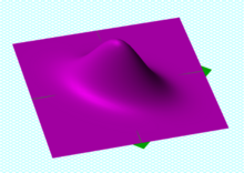
Covariance mapping[edit]
In covariance mapping the values of the  or
or  matrix are plotted as a 2-dimensional map. When vectors and are discrete random functions, the map shows statistical relations between different regions of the random functions. Statistically independent regions of the functions show up on the map as zero-level flatland, while positive or negative correlations show up, respectively, as hills or valleys.
In practice the column vectors  , and are acquired experimentally as rows of samples, e.g.
![{displaystyle [mathbf {X} _{1},mathbf {X} _{2},...mathbf {X} _{n}]={begin{bmatrix}X_{1}(t_{1})&X_{2}(t_{1})&cdots &X_{n}(t_{1})\\X_{1}(t_{2})&X_{2}(t_{2})&cdots &X_{n}(t_{2})\\vdots &vdots &ddots &vdots \\X_{1}(t_{m})&X_{2}(t_{m})&cdots &X_{n}(t_{m})end{bmatrix}},}](https://wikimedia.org/api/rest_v1/media/math/render/svg/be824f93648e01daa17bd4e9d99b4398026b0149)
where  is the i-th discrete value in sample j of the random function
  . The expected values needed in the covariance formula are estimated using the sample mean, e.g.

and the covariance matrix is estimated by the sample covariance matrix

where the angular brackets denote sample averaging as before except that the Bessel’s correction should be made to avoid bias. Using this estimation the partial covariance matrix can be calculated as

where the backslash denotes the left matrix division operator, which bypasses the requirement to invert a matrix and is available in some computational packages such as Matlab.[10]

Figure 1: Construction of a partial covariance map of N2 molecules undergoing Coulomb explosion induced by a free-electron laser.[11] Panels a and b map the two terms of the covariance matrix, which is shown in panel c. Panel d maps common-mode correlations via intensity fluctuations of the laser. Panel e maps the partial covariance matrix that is corrected for the intensity fluctuations. Panel f shows that 10% overcorrection improves the map and makes ion-ion correlations clearly visible. Owing to momentum conservation these correlations appear as lines approximately perpendicular to the autocorrelation line (and to the periodic modulations which are caused by detector ringing).
Fig. 1 illustrates how a partial covariance map is constructed on an example of an experiment performed at the FLASH free-electron laser in Hamburg.[11] The random function is the time-of-flight spectrum of ions from a Coulomb explosion of nitrogen molecules multiply ionised by a laser pulse. Since only a few hundreds of molecules are ionised at each laser pulse, the single-shot spectra are highly fluctuating. However, collecting typically  such spectra,
  , and averaging them over
  produces a smooth spectrum
  , which is shown in red at the bottom of Fig. 1. The average spectrum
  reveals several nitrogen ions in a form of peaks broadened by their kinetic energy, but to find the correlations between the ionisation stages and the ion momenta requires calculating a covariance map.
In the example of Fig. 1 spectra and  are the same, except that the range of the time-of-flight
  differs. Panel a shows
  , panel b shows
  and panel c shows their difference, which is (note a change in the colour scale). Unfortunately, this map is overwhelmed by uninteresting, common-mode correlations induced by laser intensity fluctuating from shot to shot. To suppress such correlations the laser intensity
  is recorded at every shot, put into and is calculated as panels d and e show. The suppression of the uninteresting correlations is, however, imperfect because there are other sources of common-mode fluctuations than the laser intensity and in principle all these sources should be monitored in vector . Yet in practice it is often sufficient to overcompensate the partial covariance correction as panel f shows, where interesting correlations of ion momenta are now clearly visible as straight lines centred on ionisation stages of atomic nitrogen.
Two-dimensional infrared spectroscopy[edit]
Two-dimensional infrared spectroscopy employs correlation analysis to obtain 2D spectra of the condensed phase. There are two versions of this analysis: synchronous and asynchronous. Mathematically, the former is expressed in terms of the sample covariance matrix and the technique is equivalent to covariance mapping.[12]
See also[edit]
- Covariance function
- Multivariate statistics
- Lewandowski-Kurowicka-Joe distribution
- Gramian matrix
- Eigenvalue decomposition
- Quadratic form (statistics)
- Principal components
References[edit]
- ^ a b c Park,Kun Il (2018). Fundamentals of Probability and Stochastic Processes with Applications to Communications. Springer. ISBN 978-3-319-68074-3.
- ^ William Feller (1971). An introduction to probability theory and its applications. Wiley. ISBN 978-0-471-25709-7. Retrieved 10 August 2012.
- ^ Wasserman, Larry (2004). All of Statistics: A Concise Course in Statistical Inference. ISBN 0-387-40272-1.
- ^ Taboga, Marco (2010). «Lectures on probability theory and mathematical statistics».
- ^ Eaton, Morris L. (1983). Multivariate Statistics: a Vector Space Approach. John Wiley and Sons. pp. 116–117. ISBN 0-471-02776-6.
- ^ a b W J Krzanowski «Principles of Multivariate Analysis» (Oxford University Press, New York, 1988), Chap. 14.4; K V Mardia, J T Kent and J M Bibby «Multivariate Analysis (Academic Press, London, 1997), Chap. 6.5.3; T W Anderson «An Introduction to Multivariate Statistical Analysis» (Wiley, New York, 2003), 3rd ed., Chaps. 2.5.1 and 4.3.1.
- ^ Lapidoth, Amos (2009). A Foundation in Digital Communication. Cambridge University Press. ISBN 978-0-521-19395-5.
- ^ Brookes, Mike. «The Matrix Reference Manual».
- ^ Shir, O.M.; A. Yehudayoff (2020). «On the covariance-Hessian relation in evolution strategies». Theoretical Computer Science. Elsevier. 801: 157–174. doi:10.1016/j.tcs.2019.09.002.
- ^ L J Frasinski «Covariance mapping techniques» J. Phys. B: At. Mol. Opt. Phys. 49 152004 (2016), open access
- ^ a b O Kornilov, M Eckstein, M Rosenblatt, C P Schulz, K Motomura, A Rouzée, J Klei, L Foucar, M Siano, A Lübcke, F. Schapper, P Johnsson, D M P Holland, T Schlatholter, T Marchenko, S Düsterer, K Ueda, M J J Vrakking and L J Frasinski «Coulomb explosion of diatomic molecules in intense XUV fields mapped by partial covariance» J. Phys. B: At. Mol. Opt. Phys. 46 164028 (2013), open access
- ^ I Noda «Generalized two-dimensional correlation method applicable to infrared, Raman, and other types of spectroscopy» Appl. Spectrosc. 47 1329–36 (1993)
Further reading[edit]
- «Covariance matrix», Encyclopedia of Mathematics, EMS Press, 2001 [1994]
- «Covariance Matrix Explained With Pictures», an easy way to visualize covariance matrices!
- Weisstein, Eric W. «Covariance Matrix». MathWorld.
- van Kampen, N. G. (1981). Stochastic processes in physics and chemistry. New York: North-Holland. ISBN 0-444-86200-5.
| About |
| Home |
| RO method |
| News Archive |
| Contact |
| Search |
| Documentation |
| Product Documents |
| Publications |
| ROM SAF Reports |
| Visiting Scientist |
| User Workshops |
| Data & Software |
| Product Archive |
| Product Quality |
| Browse Occultations |
| NRT Monitoring |
| Climate Monitoring |
| Software |
| User Service |
| Helpdesk |
| Helpdesk History |
| RSS Feeds |
| Registration |
| Login |
Error Covariance Matrices
The error covariance matrix (ECM) is a dataset that specifies the correlations in the observation errors between all possible pairs of vertical levels. It is given as a two-dimensional array, of size NxN , where N is the number of vertical levels in the sounding data products.
Specifically, the ECM for variable X
is given by E[(X
— E[X])(X — E[X])T],
where in practice the expectation value is estimated by an average
over a representative sample. It is a matrix because levels
are treated independently: X
is a vector of length equal to the number of vertical levels.
X could be an observation (refractivity N or bending angle α), in which case the ECM is sometimes called O,
or a
background state ({T, q, p*} for ECMWF-like models; {p, q} for Met
Office-like models), in which case the ECM is sometimes called B. Both need to be specified in the minimisation of the usual 1dvar cost function
J(x) = ½(x-b)TB-1(x-b) + ½(H(x)-y)TO-1(H(x)-y))
which is needed to produce a retrieved analysis x.
ECMs are positive semi-definite matrices which can be factorised as
ECM = DT C D
where the diagonal matrix D comprises the standard deviations of X, and defines the «size» of the variance, while the correlation matrix C describes the «shape» of the variance of X. By definition of standard deviation, the diagonal terms of C are all equal to 1.
The ROPP user has a choice of whether to use fixed standard deviations D,
read from an auxiliary covariance file, or to allow them to vary
profile-by-profile, by including them in the observation or background
file. At present, correlations C can only be read from the same auxiliary file. It is the content of these auxiliary covariance files which is described here.
In ROPP, the correlations in the covariance files are stored in packed,
«triangular» format, so that successive elements of the variable «corr»
hold the following matrix elements:
| 1 | 2 | 4 | 7 | … |
| 3 | 5 | 8 | … | |
| 6 | 9 | … | ||
| 10 | … | |||
| … |
By exploiting the symmetry of the correlation coefficients, only ½N(N+1) of them need to be stored.
The correlation matrices can be binned (in the same file) according to
latitude. In principle this could be extended to seasonality. Standard
deviations can also be held in the same file. These, rather than the
profile-by-profile SDs, will be used in the retrieval if
bg/obs_covar_method = FSFC or FSDC.
Further details on all the above can be found in the ROPP FM and 1DVAR User Guide.
Below, there are error-covariance matrices for the following:
- Covariance matrices for NRT products
- Covariance matrices for Reprocessed climate data records
- Other covariance matrices (included in ROPP)
Each matrix can be provided in several versions reflecting variations with geographical areas (e.g. latitude) and with season.
Covariance matrices for NRT products
| Description | Image (click to expand) |
File |
| Background
Suitable for 137L ECMWF background state. Currently, the T and p* standard deviations are the ones The block diagonal structure of correlation matrix arises |
 |
ropp_bg_ecmwf_error_corr_L60.nc
ropp_bg_ses_ecmwf_error_corr_L137.nc |
| ObservationsSuitable for 247L refractivity retrievals. (Bending angle correlation matrices are usually assumed to be diagonal.) Note that there is a minimum σ(N) of 0.02 N-units above |
 |
ropp_ob_refrac_error_corr_247L.nc |
Covariance matrices for Reprocessed climate data records
| Description | Image (click to expand) |
File |
| Background
Suitable for 60 L ERA-I background profiles. Average of |
 |
ropp_bg_ecmwf_error_corr_L60.nc
bg_ef_ei_error_corr_sigma_PsBias_LatB5d_L60.nc |
Other covariance matrices (included in ROPP)
Some example ECMs are available in the ropp_1dvar/errors directory of the ROPP distribution, for the benefit of the users. They are described below.
| Description | Image (click to expand) |
File |
| Background Suitable for (early) 60L ECMWF background state {T, q, p*}. Note that correlation matrix assumes level 1 at the top of the atmosphere. |
 |
ropp_bg_ecmwf_error_corr_L60.nc |
| Background Suitable for (current) 91L ECMWF background state {T, q, p*}. Note that correlation matrix assumes level 1 at the bottom of the atmosphere. |
 |
ropp_bg_ecmwf_error_corr_L91.nc |
| BackgroundSuitable for (early) 50L Met Office background state {p, q}. Three latitude bands: -90 to -20, -20 to 20, 20 to 90N. |

|
ropp_bg_meto_error_corr_L50.nc |
| BackgroundSuitable for (current) 70L Met Office background state {p, q}. Three latitude bands: -90 to -20, -20 to 20, 20 to 90N. |

|
ropp_bg_meto_error_corr_L70.nc |
| Observation
Suitable for 300L bending angles. (Note that the correlation matrix C is the identity matrix). |
 |
ropp_ob_bangle_error_corr.nc |
| Observation
Suitable for standard 247L refractivities. |
 |
ropp_ob_refrac_error_corr.nc |


|
EUMETSAT ROM SAF licence
|
|

|

|
|
Copyright © 1999-2023 EUMETSAT
|

Battery state-of-power evaluation methods
Shunli Wang, … Zonghai Chen, in Battery System Modeling, 2021
7.4.4 Main charge-discharge condition test
The initial value of the error covariance matrix P0 can be determined from the X0 error of the initial state. In the application, the initial value should be as small as possible to speed up the tracking speed of the algorithm. Two important parameters are processed noise variance matrix Q and observation noise variance matrix R. As can be known from theoretical formula derivation, the dispose to Q and R plays a key role in improving the estimation effect by using this algorithm. Because it affects the size of the Kalman gain matrix K directly, the value of error covariance matrix P can be described as shown in Eq. (7.61):
(7.61)Rk=Eυk2=συ2
It is the expression of the observation noise variance, which is mainly derived from the distribution of observation error of experimental instruments and sensors, as shown in Eq. (7.62):
(7.62)Qk=Eω1k2Eω1kω2kEω2kω1kEω2k2=σω1,12σω1,22σω2,12σω2,22
It is the relationship between the system noise variance and the processing noise covariance. The two states in the system are generally unrelated and the covariance value is zero. Therefore, the diagonal variance can have a small value. The variance Q of processing noise is mainly derived from the error of the established equivalent model, which is difficult to be obtained by theoretical methods or means. A reasonable value range can be obtained through continuous debugging through simulation, and it is usually a small amount.
To verify the applicable range and stability of the algorithm, the input of different working conditions is used to observe the estimation accuracy of the algorithm. In this simulation, two working conditions are used: the constant-current working condition and the Beijing bus dynamic street test working condition. For the constant-current condition, only a constant value needs to be set in the program. To increase the complexity of the condition, two shelved stages are added to the constant-current input list to verify the tracking effect of Ah and the extended Kalman filtering. The following code is generated for the current.
The experimental data should be used to simulate the algorithm under its operating conditions. The current input module is realized in the environment under Beijing bus dynamic street test operating conditions. It is the time integration module, whose output is the capacity change of the working condition, and the lower part is the working condition data output module. It outputs the current into the workspace at the minimum time interval of the sampling measurement. The data onto the workspace are a time-series type and the current data need to be extracted. The data extraction and transformation can be performed in the main program, wherein the working condition is the Simulink module. The current is the time-series data, including the current output. S_Est is the algorithm program module, whose input is the initial S_Est_init and current data onto the estimated state value.
The current data are input into the program module of the extended Kalman filtering algorithm based on the model, and the initial values of other parameters have been determined in the program. The program finally outputs the ampere hour time integral and the state estimation curve of the extended Kalman filtering through the minimum time interval of 10 times as the sampling time. The current curve of the experimental test can be obtained as shown in Fig. 7.13.

Fig. 7.13. Pulse current operating current curve for the experimental test. (A) Main charge working condition. (B) Main discharge experimental test.
The unscented Kalman filtering algorithm is programmed by writing scripts to realize algorithm simulation to compare the output effect. The specific implementation process conforms to the processing requirements, and the main simulation program can be constructed. The program takes 10 times the minimum time interval as the sampling time and simulates the three methods of the state estimation, including ampere hour time integration, extended Kalman filtering, and unscented Kalman filtering, to compare the following situation of the three methods of the state over time. The program simultaneously outputs the state variation curve and estimation error curve with time, so that the tracking effect and error variation on the three methods can be obtained visually. Its implementation process is consistent with script. Different modules are used to replace the code block. The integration advantage of the environment is used in the graphical interface to obtain the same stimulation effect.
The operation logic is ensured by the unchanged intuitive presentation of the calculation process. Based on script implementation, the modular simulation is built accordingly. The experiment data are used as the input current, and the state prediction is obtained by the state prediction module. The forecast and model parameters are calculated. After that, the equivalent model can be used to predict the completion status value of Up as well as the output voltage. The input of the algorithm includes the update module, output state correction, and error covariance matrix update as the basis of the forecast. It takes the ampere hour integral result as the minimum time interval of the current data, which is taken as the reference value of the measured state.
The estimation effect of ampere hour and extended Kalman filtering is compared when the minimum time interval can be set as 10 times as the sampling period. The stability of the extended Kalman filtering algorithm is evaluated under working conditions. The state variable needs to accept the last estimated value as the basis of the next state prediction, in which the predicted value Up_pre is directly input into the corresponding position of the resistance-capacitance circuit modeling to conduct the terminal voltage prediction of the current polarization voltage. The functions of each part are realized in a more modular way for the complete structure and clear hierarchy.
Read full chapter
URL:
https://www.sciencedirect.com/science/article/pii/B9780323904728000044
Dynamic Model Development
P.W. Oxby, … T.A. Duever, in Computer Aided Chemical Engineering, 2003
3.2 An Optimality Property of the Determinant Criterion
Equation (12) can be generalized by replacing the inverse of the estimate of the error covariance matrix,
Σ^εn−1, with an arbitrary symmetric positive definite weight matrix, W:
(14)Δθ^(k)=(XTWX)−1XTWz(θ^(k))
The estimate of the parameter covariance is:
(15)Σ^θ=(XTWX)−1XTWΣ^εn(XTWX)−1
If the determinant of the estimate of the parameter covariance matrix,
|Σ^θ|, is minimized with respect to the elements of W, the solution is independent of X and is simply
(16)W=Σ^εn−1
Substitution of (16) back into (14) gives (12) which, as has been shown, is equivalent to the determinant criterion. Therefore of all weighting schemes in the form of (14), it is the one equivalent to the determinant criterion that minimizes
|Σ^θ|, the determinant of the estimate of the parameter covariance matrix when the error covariance is unknown. This appears to be a rather strong result in support of the determinant criterion. It might also be noted that, unlike derivations based on likelihood, this result does not depend on the measurement errors being normally distributed. But it will be shown that the practical usefulness of the result does depend on the assumption that the residual covariance
Z(θ^)Z(θ^)T/n, is a good estimate of the true error covariance. Ideally one would want W to be the inverse of the error covariance matrix. The determinant in effect makes a compromise and substitutes an estimate of it. The potential problem here is that if the data set is not large, the residual covariance matrix may be a poor estimate of the error covariance matrix. A poor estimate of the error covariance matrix will lead to a poor estimate of the parameter covariance matrix. Therefore, although the determinant criterion gives the minimum determinant of the estimate of the parameter covariance matrix, if this estimate is poor, then the optimality property may be of little significance. This suggests that the optimality of the determinant criterion may be more relevant for large data sets than small ones. The simulation studies presented in Section 4 will confirm this to be true.
Read full chapter
URL:
https://www.sciencedirect.com/science/article/pii/S1570794603800706
Kalman Filters and Nonlinear Filters
Vytas B. Gylys, in Encyclopedia of Physical Science and Technology (Third Edition), 2003
IV.B Square Root Filtering
By far the greatest trouble spot in computer mechanization of the KF is the updating of state error covariance matrix P, that is, the computation of Pk∣k according to Eq. (18). As the estimation process progresses, the elements of Pk∣k typically continue to decrease in magnitude and so matrix Pk∣k keeps approaching the zero matrix, although theoretically it should forever remain positive definite, no matter how small in magnitude its elements become. Hence, unless special measures are taken, accumulation of roundoff error in the repetitive use of Eq. (18) may cause the computed Pk∣k to lose its positive definiteness. As suggested by the matrix inversion operation appearing on the right-hand side of Eq. (16) for computing the Kalman gain, this situation is aggravated if several components of the measurement vector are very accurate and consequently the positive definite measurement error covariance matrix R is ill conditioned, that is, if R has eigenvalues of both relatively very large and small magnitudes.
Let A be a nonnegative definite symmetric matrix; then there exists a matrix S such that A = SST. Matrix S is often called the square root of A. The Cholesky decomposition algorithm provides a method of constructing from A the matrix S so that S is lower triangular; that is, all elements of S above the main diagonal are zero. Square root filtering is motivated by the observations that, if the state error covariance matrix P = SST, then (a) since SST is always nonnegative definite, matrix P expressed as SST cannot become negative definite, and (b) matrix S is generally less ill conditioned than matrix P.
Several versions of the square root filtering algorithm are known. The earliest form was developed by J. E. Potter in 1964 for applications in which the process noise is absent (i.e., covariance matrix Q is zero) and the measurements are sequentially processed as scalars. In 1967 J. F. Bellantoni and K. W. Dodge extended Potter’s results to vector-valued measurements. A. Andrews in 1968 and then S. F. Schmidt in 1970 published two alternative procedures for handling the process noise. In 1973 N. A. Carlson described a procedure that considerably improved the speed and decreased the memory requirements of square root filtering and in which, as in Potter’s algorithm, vector-valued measurements are processed sequentially as scalars. Finally, the so-called UDUT covariance factorization method is the most recent major milestone in numerical handling of KFs. This method, developed by G. J. Bierman and C. L. Thornton, represents the state error covariances before and after the measurement update step asPk|k−1=Uk|k−1Dk|k−1Uk|k−1TandPk|k=Uk|kDk|kUk|kT,with D being a diagonal matrix and U an upper triangular matrix with 1’s on its main diagonal. In this method, the square root of the covariance matrix, which now would correspond to UD1/2, is never computed explicitly, which avoids numerical computation of square roots. Like Carlson’s algorithm, the UDUT factorization method maintains the covariance matrix in factored form and so (like Carlson’s algorithm) is considerably more efficient in processor time and storage than the original Potter algorithm.
As a quick comparison of computational efficiency, the conventional Kalman method, the less efficient form of Carlson’s algorithm, and the UDUT factorization method are roughly equal: The processing of each time step (consisting of one time propagation and one measurement update) requires of the order of 16[9ns3 + 9ns2nm + 3ns2nw] adds and about the same number of multiplies, plus a relatively modest number of divides and square roots (square roots are required only in some, as in Potter’s or Carlson’s square root algorithms). Here, as before, ns is the length of the state vector, nm the length of the measurement vector, and nw the lenght of the process noise vector w. The faster version of Carlson’s algorithm is more efficient and requires only of the order of 16[5ns3 + 9ns2nm + 3ns2nw] adds and 16[5ns3 + 12ns2nm + 3ns2nw] multiplies, plus 2nsnm divides and nsnm square roots, at each time point. The stable (Joseph) form of the KF [as given by Eq. (18′)] fares more poorly: At each time step, it requires of the order of 16[18ns3 + 15ns2nm + 3ns2nw] adds and about the same number of multiplies.
As a summary, (a) a square root filter is a numerically stable form for performing the KF covariance–gain processing defined by Eqs. (15), (16), and (18); (b) the efficiency of its more recent versions roughly compares with that of these three equations; (c) the increased stability allows one to use relatively low-precision arithmetic in the KF gain–covariance processing, with a possible exception of some dot products.
Real-time implementation of a filter involves additional issues that are unimportant in the non-real-time environment. Besides the adequacy of functional performance, the most important of these issues is the requirement to produce timely responses to external stimuli. Thus, resorting to a parallel or concurrent processing may be the only way out. This usually implies the use of special hardware architectures such as parallel, vector pipelined, or systolic processors.
As one example, consider the use of a filter in the tracking of multiple objects in a hard real-time environment characterized by strict deadlines. In such a case one may want to maintain simultaneously many estimation processes, each handling a single object. Parallel processors may seem to be a suitable hardware architecture for this problem, but if separate estimation processes in such an application progress at different rates and at any time some of them require a great amount of special handling, then parallel architecture, such as a single-instruction multiple-data stream computer, may not be the best choice. As another example, consider a KF to be implemented as part of a navigation system on a small airborne computer (uniprocessor). Suppose that the navigation measurements come at a certain fixed rate. If the filtering process cannot keep up with the arrival rate of measurements and so not all of them can be utilized, the estimation performance may deteriorate. In this problem, if there is an upper bound on hardware resources, the only solution may be to decompose the estimation algorithm into concurrently executable processes. For instance, the time-propagation step (which, say, is to be executed at a relatively high rate) may constitute one process and the measurement-update step (which needs to be executed only at some lower rate, say, at the rate of measurement arrivals) may constitute another. Such a decomposition of an estimation algorithm into concurrent procedures often creates a surrogate algorithm that performs more poorly than the original algorithm.
The effects of the finite-length word computing is another issue that must be considered in filter implementation for real-time applications. The computer on which a filter is developed and validated through successive off-line simulations is often more powerful and uses higher-precision arithmetic and number representations than the ultimate real-time processor. Hence, one must in advance determine in advance what effect a shorter word length will have on performance.
Read full chapter
URL:
https://www.sciencedirect.com/science/article/pii/B0122274105003574
Computer Techniques and Algorithms in Digital Signal Processing
K. Giridhar, … Ronald A. Iltis, in Control and Dynamic Systems, 1996
A Appendix – Time Updates for the Blind MAPSD Algorithm
In this Appendix, we derive the one-step time updates of the channel estimate and the associated error covariance matrix for the blind MAP symbol detector developed in Section 4.2. Recall from Eq. (51) that
(A.1)pfk+1|dik+1,Nf,rk=∑j:djk,Nf∈dik+1,Nfαjp(fk+1|djk,Nf,rk)
where αj is given by Eq. (52). Using Eq. (49), this Gaussian sum can be explicitly written as follows:
(A.2)pfk+1|dik+1,Nf,rk=∑j:djk,Nf∈dik+1,NfαjNfk+1;Ff^jk|k,FPjk|kFH+Q
which defines the one-step prediction of the mean vector f^ik+1|k and the covariance matrix Pik+1|k. Some basic results about sums of Gaussian p.d.f.s can be used to derive these one-step predictions.
Lemma: Let the p.d.f. of the random vector x be a weighted sum of N multivariate Gaussian p.d.f.s as follows:
(A.3)px=∑j=1NαjNx;xj,Pj
where αj , xj, and Pj are, respectively, the jth weight, mean, and covariance. (i) The mean value of x is given by
(A.4)xa=∑j=1Nαjxj.
(ii) The error covariance is given by
(A.5)Pa=∑j=1NαjPj+xa–xjxa–xjH.
Proof: The first part of the lemma is easily proved from the definition of xa, i.e.,
(A.6)xa=Ex=∫xx∑j=1NαjNx;xj,Pjdx=∑j=1Nαjxj.
To prove the second part of the lemma, consider
(A.7)Pa=Ex−xax−xaH=∑j=1Nαj∫xxxHNjdx+xaxaH−∫xxxaHNjdx−∫xxaxHNjdx
where, for convenience, we have used the notation Nj to represent the p.d.f. N(x; xj, Pĵ). Observe that ∫xxaHNjdx=xjxaHand∫xaxHNjdx=xaxjH. By adding and subtracting the term xjxjH to the expression inside the square brackets, we obtain
(A.8)Pa=∑j=1Nαj∫xxxHNjdx−xjxjH+xaxaH−xjxaH−xaxjH+xjxjH=∑j=1Nαj∫xxxHNjdx−xjxjH+xa−xjxa−xjH..
It is straightforward to show that
(A.9)∑j=1Nαj∫xxxHNjdx−xjxjH=∑j=1Nαj∫xx−xj(x−xj)HNjdx=∑j=1NαjPj.
Substituting this result into Eq. (A.8 ), we obtain the result in Eq. (A.5 ) for the error covariance Pa, which completes the proof.
To obtain the one-step predicted mean vector of the blind MAPSD algorithm, Eq. (A.4 ) is used with xj=Ff^jk|k. The summation is performed over the M predecessor subsequences djk,Nf, yielding
(A.10)f^ik+1|k)=∑j:djk,Nf∈dik+1,NfαjFf^jk|k.
By substituting αj=pdjk,Nf|rk−1/qik, the final expression in Eq. (53) is obtained. Similarly, the one-step error covariance update in Eq. (54) is obtained by substituting FPjk|kFH+Q=Pj and
(A.11)νj,ikνj,iHk=xa−xjxa−xjH
into Eq. (A.5 ) where xa=f^ik+1|k (and xj=Ff^jk|k as above).
Read full chapter
URL:
https://www.sciencedirect.com/science/article/pii/S0090526796800454
State Estimation
Jay Farrell, in The Electrical Engineering Handbook, 2005
4.3 Recursive State Estimation
Equations 4.4 through 4.5 provide the mean and the covariance of the state through time based only on the initial mean state vector and its error covariance matrix. When measurements y(k) are available, the measurements can be used to improve the accuracy of an estimate of the state vector at time k. The symbols xˆ−(k) and xˆ+(k) are used to denote the estimate of x(k) before and after incorporating the measurement, respectively.
Similarly, the symbols Pxˆ−(k) and Pxˆ+(k) are used to denote the error covariance matrices corresponding to xˆ−(k) and xˆ+(k), respectively. This section presents the time propagation and measurement update equations for both the state estimate and its error covariance. The equations are presented in a form that is valid for any linear unbiased measurement correction. These equations contain a gain matrix K that determines the estimator performance. The choice of K to minimize the error covariance Pxˆ+(k) will be of interest.
For an unbiased linear measurement, the update will have the form:
(4.8)xˆ+(k)=xˆ−(k)+K(k)(y(k)−yˆ−(k)),
where yˆ−(k)=H(k)xˆ−(k).. The error covariance of xˆ+(k) is the following:
(4.9)Pxˆ+(k)=(I−K(k)H(k))Pxˆ−(k)(I−K(k)H(k))T +K(k)R(k)KT(k).
K(k) is a possibly time-varying state estimation gain vector to be designed. If no measurement is available at time k, then K(k) = 0, which yields xˆ+(k)=xˆ−(k) and Pxˆ+(k)=Pxˆ−(k). If a measurement is available, and the state estimator is designed well, then Pxˆ+(k)≤Pxˆ−(k). In either case, the time propagation of the state estimate and its error covariance matrix is achieved by:
(4.10)xˆ−(k+1)=Φ(k)xˆ+(k)+Γˆuu(k)
(4.11)Pxˆ−(k+1)=Φ(k)Pxˆ+(k)ΦT(k)+ΓωQd(k)ΓωT.
At least two issues are of interest relative to the state estimation problem. First, does there exist a state estimation gain vector K(k) such that xˆ is guaranteed to converge to x regardless of initial condition and the sequence u(k)? Second, how should the designer select the gain vector K(k)?
The first issue raises the question of observability. A linear time-invariant system is observable if the following matrix has rank n:
[HT, ΦTHT, …,( ΦT)nHT].
When a system is observable, then it is guaranteed that a stabilizing gain vector K exists. Assuming that the system of interest is observable, the remainder of this chapter discusses the design and analysis of state estimators.
Figure 4.1 portrays the state estimator in conjunction with the system of interest. The system of interest is depicted in the upper left. The state estimator is superimposed on a gray background in the lower right.

FIGURE 4.1. State Estimation System Block Diagram
This interconnected system will be referred to as the state estimation system. The figure motivates several important comments. First, although the state estimator has only n states, the state estimation system has 2n states. Second, the inputs to the state estimation system are the deterministic input u and the stochastic inputs ω and v. Third, the inputs to the state estimator are the deterministic input u and the measured plant output y. The state space model for the state estimation system is the following:
(4.12)[x(k+1)xˆ−(k+1)]=[Φx0LHxΦ−LH][x(k)xˆ−(k)]+[ΓuΓω0Γˆu0L][u(k)ω(k)v(k)],
where L = ΦK.
Based on this state-space model, with the assumption that the system is time invariant, the transfer function from v to yˆ is as written here:
(4.13)Gv(z)=H[zI−(Φ−LH)]−1L,
where z is the discrete-time unit advance operator. Assuming that H = Hx, the transfer function from u to r is as follows:
(4.14)Gu(z)=H[zI−(Φ−LH)]−1 [(zI−Φ)(zI−Φx)−1Γu−(zI−Φx)(zI−Φx)−1Γˆu].
Therefore, if Γu=Γˆu and Φx = Φ, then this transfer function is identically zero. Assuming again that H = Hx, the transfer function from ω to r is the following:
(4.15)Gω(z)=H[zI−(Φ−LH)]−1[zI−Φ][zI−Φx]−1Γω.
In the special case where, in addition, Φx = Φ, the transfer function Gω(z) has n identical poles and zeros. This transfer functions is often stated as:
(4.16)Gω(z)=H[zI−(Φ−LH)]−1Γω,
where n pole and zero cancellations have occurred. These pole-zero cancellations and therefore the validity of equation 4.16 are dependent on the exact modeling assumption and the stability of the canceled poles.
Read full chapter
URL:
https://www.sciencedirect.com/science/article/pii/B9780121709600500815
Data Assimilation in Numerical Weather Prediction and Sample Applications
Andrew S. Jones, Steven J. Fletcher, in Solar Energy Forecasting and Resource Assessment, 2013
13.3.5 Ensemble DA
The ensemble Kalman filter (EnsKF) is a sequential filter that forecasts the state vector, xf, as well as the model-error covariance matrix, Pf, toward a future time step (Evensen, 1994). This is a linear process, but it can employ nonlinear models within the system; no adjoints are required. For example, the forward state is given by the propagation of the model forward in time
(13.29)xf(ti)=Mi−1[xa(ti−1)]
as well as its associated forecast-error covariance matrix
(13.30)Pf(ti)=Mi−1Pa(ti−1)Mi−1T+Q(ti−1)
This is followed by an analysis step that updates (or readjusts) the state information and the forecast-error covariance information
(13.31)xa(ti)=xf(ti)+Kidi
(13.32)Pa(ti)=(I−KiHi)Pf(ti)
where the innovation vector, di, is given by
(13.33)di=yio−Hi[xf(ti)]
It is important to note that M and H are linearizations of the gradients of M and H with respect to the control vector, x. The Kalman gain, Ki, is given by
(13.34)Ki=Pf(ti)HiT[HiPf(ti)HiT+Ri]−1
where Pf(ti) is now approximated by the mean ensemble estimate
(13.35)Pf(ti)≈1K−2∑K≠lK[xf(tk)−x¯f(tl)][xf(tk)−x¯f(tl)]T
K is the number of ensemble-model runs required to generate the estimate, and a reference model state, l, is used to define the mean ensemble estimate of the forecast error covariance matrix. In addition to the approach in equation 13.35, other EnsKF variants are used by the NWP DA community. The analysis stage that propagates the forecast error covariance matrix is a powerful feature of EnsKF. Additional improvements in EnsKF performance can be achieved by improving sampling behaviors—for example, using sampling strategies and square root schemes, some of which also allow for a low-rank representation of the observational-error covariance matrix (Evensen, 2004).
Read full chapter
URL:
https://www.sciencedirect.com/science/article/pii/B9780123971777000139
The Basics of Analytical Mechanics, Optimization, Control and Estimation
Kyle T. Alfriend, … Louis S. Breger, in Spacecraft Formation Flying, 2010
3.8 Kalman Filtering
In 1960, Robert Kalman introduced a new approach for minimum mean-square error filtering that used state-space methods [80]. The Kalman Filter (KF) is a recursive scheme that propagates a current estimate of a state and the error covariance matrix of that state forward in time. The filter optimally blends the new information introduced by the measurements with old information embodied in the prior state with a Kalman gain matrix. The gain matrix balances uncertainty in the measurements with the uncertainty in the dynamics model. The KF is guaranteed to be the optimal filter (in the sense of minimizing the 2-norm-squared of the estimation error) for a linear system with linear measurements [81]. However, few systems can be accurately modeled with linear dynamics. Shortly after its inception, improvements on the Kalman filter to handle nonlinear systems were proposed. One of the most popular choices, the Extended Kalman Filter (EKF), was applied to relative navigation filters in LEO [43]. We will demonstrate how to use the EKF for relative spacecraft state estimation in Chapter 12.
The discrete EKF is as a state estimator for systems whose state dynamics model, measurement model, or both may be nonlinear, as in Eqs. (3.48) and (3.53) [81]. The dynamics model provides the equations to propagate xˆk, the estimate of the state x at time k, to time step k+1, producing xˆk+1. The measurement model then incorporates the new sensor information to update this estimate, updating the a priori estimate xˆk+1− to the a posteriori estimate, xˆk+1+. This process is illustrated in Fig. 3.1.

FIGURE 3.1. A Kalman filter process.
The continuous state x is governed by the dynamics
(3.48)ẋ(tk)=f(x,u,tk)+w(tk)
where u is a known control input, and w(t) is an additive white noise that models the error accumulated by uncertainty in the dynamics during the time step. The power spectral density of this zero mean, white noise process is
(3.49)Q=E[w(t)w(t)T]
To proceed, linear expressions for the dynamics and measurement equations must be formed. In general, this requires knowledge of the probability density function [81], but the EKF approximates the nonlinear function by expanding it in a Taylor series, at each time step, about the current estimate,
(3.50)Fk=∂f∂x|x=xˆk
The dynamics are discretized with time step Δt by forming the state transition matrix,
(3.51)Φk=eFkΔt
The cumulative effect of the white noise process w(t) over the time step is captured in the discrete process noise covariance matrix
(3.52)Qk=∫0ΔteFkτQ(eFkτ)Tdτ
The vector of measurements, y,
(3.53)y=h(x,t)+vk
is modeled as a nonlinear function of the state and time, with an additive white noise process v(t) that accounts for uncertainty in the sensors and their models. The measurement noise covariance matrix is defined by
(3.54)Rk=E[vkvkT]
The nonlinear measurement equation is also linearized about the current estimate,
(3.55)Hk=∂h∂x|x=xˆk−
Because approximations must be made in the linearization, the EKF is a suboptimal filter, in the sense that its stability and performance are not guaranteed. Fortunately, the dynamics of orbital motion are fairly simple, and the EKF can have very good performance in space navigation applications. The discrete, linear representation of the system dynamics are
(3.56)xk=Φk−1xk−1+wk−1+uk−1
The confidence in the current estimate is captured in the state error covariance matrix, P,
(3.57)Pk=E[x̃kx̃kT]=E[(xˆk−xk)(xˆk−xk)T]
where x̃k=xˆk−xk is the estimation error. The first step in the EKF involves propagating the state and error covariance forward in time. Equation (3.56), with zero process noise, is used to propagate the state estimate. The error covariance is propagated forward using
(3.58)Pk−=Φk−1Pk−1+Φk−1T+Qk−1
An alternate approach to the time propagation step involves using the nonlinear dynamics equations to propagate the state. A 4th-order Runge–Kutta integration scheme uses the nonlinear state dynamics equation
(3.59)xˆ̇(t)=f(xˆ(t),u(t))for t=tk−1→tk
to find xˆk. The state covariance is still propagated with Eq. (3.58), so the state transition matrix Φk−1 must be calculated regardless of whether the linear or nonlinear state propagation is chosen.
The second step of the filter uses the measurement equation to update the a priori state xˆk− to the a posteriori state xˆk+. When a measurement becomes available, the new information provided by the measurement and the previous information captured in the state estimate are combined to form an updated state estimate. The Kalman gain K is the blending gain matrix that is used to weight the importance of the old and new information. The optimum gain matrix is formulated by minimizing the trace of the a posteriori state error covariance matrix Pk+, which essentially minimizes the estimation error vector at each time step [81]. The terms in the gain matrix equation include the previous state estimate, the linearized measurement matrix, and the expected noise of the new measurements,
(3.60)Kk=Pk−HkT(HkPk−HkT+Rk)−1
The nonlinear measurement equation is used to update the state estimate
(3.61)xˆk+=xˆk−−Kk(yk−hk(xˆk−))
Note that the computation of the gain matrix Kk requires the linear measurement matrix Hk. The covariance is updated after the measurement with
(3.62)Pk+=(I−KkHk)Pk−(I−KkHk)T+KkRkKkT
which is the Joseph form of the covariance update whose inherent symmetry makes it numerically stable [82].
Read full chapter
URL:
https://www.sciencedirect.com/science/article/pii/B9780750685337002086
Static State Estimation
Soliman Abdel-hady Soliman Ph.D., Ahmad M. Al-Kandari Ph.D., in Electrical Load Forecasting, 2010
2.3 Properties of Least Error Squares Estimation
Least error squares estimation results are easy to compute and possess a number of interesting properties. The least squares are the best estimates (maximum likelihood) when the measurement errors follow a Gaussian or normal distribution and the weighting matrix is equal to the inverse of the error covariance matrix. The least error squares estimates can be easily calculated.
Where the measurement error distribution does not follow a Gaussian distribution and the number of measurements greatly exceeds the number of unknown parameters, the method of least error squares yields very good estimates. However, there are many estimation problems for which the error distribution is not a Gaussian and the number of measurements does not greatly exceed the number of unknown parameters. In such cases, the least error squares estimations are adversely affected by bad data. This problem has been recognized and addressed by several researchers who have proposed different ways of refining the least error squares method to make estimation less affected by the presence of bad data. In the next section, we discuss an alternative technique to the LES estimation. This technique is based on least absolute value approximation.
Read full chapter
URL:
https://www.sciencedirect.com/science/article/pii/B9780123815439000026
Principles of meteorology and numerical weather prediction
Sue Ellen Haupt, … Branko Kosović, in Renewable Energy Forecasting, 2017
1.2.2.2 Variational assimilation
Variational assimilation techniques are a form of statistical interpolation. All statistical interpolation techniques require an estimation of the error covariances between variables in the background state, as well as error covariances between the observed variables. These techniques find the optimal analysis by globally minimizing a cost function that incorporates the distance between the analysis and observations within the assimilation window. This method also requires the observation error covariance matrix and the background error covariance matrix (e.g., Talagrand, 1997; Kalnay, 2003), which at times may be difficult to compute accurately. In three-dimensional variational DA (3D-Var) schemes, these error covariance matrices come from a static climatology, and all observations within a given assimilation window are assumed to be valid at the analysis time. These assumptions reduce the computational burden. In contrast, four-dimensional variational DA (4D-Var) schemes seek to minimize the cost function, subject to the NWP model equations, to find the best model trajectory through the entire assimilation window, rather than just at the analysis time. In addition, the error covariance matrices are flow-dependent in 4D-Var. These differences make 4D-Var significantly more computationally intensive than 3D-Var, but also more accurate (e.g., Klinker et al., 2000; Yang et al., 2009).
Read full chapter
URL:
https://www.sciencedirect.com/science/article/pii/B9780081005040000019
Smart grids: control and cybersecurity
Magdi S. Mahmoud, … Mutaz M. Hamdan, in Cyberphysical Infrastructures in Power Systems, 2022
2.2.3 Cyberattack minimization in smart grids
A recursive KF estimator (RKFE) is constructed to operate on observation information in order to produce the optimal state estimation. The forecasted system-state estimate is expressed as follows:
(2.8)xˆr(k)=Adxˆ(k−1)+Bdu(k−1),
where xˆ(k−1) is the previous state estimate. Then the forecasted error covariance matrix is given by
(2.9)Pr(k)=AdP(k−1)AdT+Qw(k−1),
where P(k−1) is the previously estimated error covariance matrix. The observation innovation residual d(k) is given by
(2.10)d(k)=yrd(k)−Cxˆr(k),
where yrd(k) is the dequantized and demodulated output bit sequence. The Kalman gain matrix can be written as
(2.11)K(k)=Pr(k)CT[CPr(k)CT+Rv(k)]−1.
This yields the updated state estimation as
(2.12)xˆ(k)=xˆr(k)−K(k)d(k),
along with the updated estimated error-covariance matrix
(2.13)P(k)=Pr(k)−K(k)CPr(k).
After estimating the system state, the proposed control strategy is applied for regulating the MG states as shown in the next section.
Read full chapter
URL:
https://www.sciencedirect.com/science/article/pii/B9780323852616000117
$begingroup$
How is the var/cov error matrix calculated by statistical analysis packages in practice?
This idea is clear to me in theory. But not in practice. I mean, if I have a vector of random variables $textbf{X}=(X_{1}, X_{2}, ldots, X_{n})^top$, I understand that the variance/covariance matrix $Sigma$ will be given the external product of the deviance-from-the-mean vectors: $Sigma=mathrm{E}left[(textbf{X}-mathrm{E}(textbf{X}))(textbf{X}-mathrm{E}(textbf{X}))^topright]$.
But when I have a sample, the errors of my observations are not random variables. Or better, they are, but only if I take a number of identical samples from the same population. Otherwise, they’re given. So, again my question is: how can a statistical package produce a var/cov matrix starting from a list of observations (i.e. a sample) supplied by the researcher?
![]()
asked Jun 24, 2013 at 14:01
![]()
$endgroup$
2
$begingroup$
The covariance matrix for a model of the type $y = Xbeta + epsilon$ is usually computed as $$(X^t X)^{-1}frac{sigma^2}{d}$$ where $sigma^2$ is the residual sum of squares, $sigma^2=sum_i (y_i — X_ihatbeta)^2$ and $d$ is the degrees of freedom (typically the number of observations minus the number of parameters).
For robust and or clustered standard errors, the product $X^t X$ is modified slightly. There may also be other ways to calculate the covariance matrix, e.g. as suggested by the expectation of outer products.
answered Jul 24, 2013 at 16:40
![]()
Simen GaureSimen Gaure
7145 silver badges7 bronze badges
$endgroup$
1
$begingroup$
- OLS estimation of the error variance, $sigma^2$:
$$s^2=frac{hat varepsilon^tophat varepsilon}{n-p}$$
This is included in Practical Regression and Anova using R
by Julian J. Faraway, page 21
.
Example of its calculation in R, based on linear model of miles-per-gallon regressed on multiple car model specs included in the mtcars database: ols = lm(mpg ~ disp + drat + wt, mtcars). These are the manual calculations and the output of the lm() function:
> rdf = nrow(X) - ncol(X)                    # Residual degrees of freedom
> s.sq = as.vector((t(ols$residuals) %*% ols$residuals) / rdf)
>                                            # s square (OLS estimate of sigma square)
> (sigma = sqrt(s.sq))                       # Residual standar error
[1] 2.950507
> summary(ols)

Call:
lm(formula = mpg ~ disp + drat + wt, data = mtcars)
...
Residual standard error: 2.951 on 28 degrees of freedom
- Variance — Covariance matrix of the estimated coefficients, $hat beta$:
$$mathrm{Var}left[hat beta mid X right] =sigma^2 left(X^top Xright)^{-1}$$
estimated as in page 8 of this online document as
$$hat{mathrm{Var}}left[hat beta mid X right] =s^2 left(X^top Xright)^{-1}$$
> X = model.matrix(ols)                             # Model matrix X
> XtX = t(X) %*% X                                  # X transpose X
> Sigma = solve(XtX) * s.sq                         # Variance - covariance matrix
> all.equal(Sigma, vcov(ols))                       # Same as built-in formula
[1] TRUE
> sqrt(diag(Sigma))                                 # Calculated Std. Errors of coef's
(Intercept)        disp        drat          wt
7.099791769 0.009578313 1.455050731 1.217156605
> summary(ols)[[4]][,2]                             # Output of lm() function
(Intercept)        disp        drat          wt
7.099791769 0.009578313 1.455050731 1.217156605
answered Jul 25, 2018 at 3:56
![]()
Antoni ParelladaAntoni Parellada
25.2k16 gold badges110 silver badges212 bronze badges
$endgroup$
$begingroup$
With linear regression we are fitting a model $Y = beta*X +varepsilon$. $Y$ is the dependent variable, the $X$’s are the predictor (explanatory) variables. We use the data provided to us (the training set or the sample) to estimate the population $beta$’s. The $X$’s are not considered random variables. The $Y$’s are random because of the error component.
![]()
answered Jun 24, 2013 at 15:05
![]()
$endgroup$
4
Least Squares Estimation
-
Ordinary Least Squares
-
Covariance-Weighted Least Squares
-
Error Covariance Estimation
-
Feasible Generalized Least Squares
-
Panel Corrected Standard Errors
Ordinary Least Squares
When you fit multivariate linear regression models using mvregress, you can use the optional name-value pair 'algorithm','cwls' to choose least squares estimation. In this case, by default, mvregress returns ordinary least squares (OLS) estimates using Σ=Id. Alternatively, if you specify a covariance matrix for weighting, you can return covariance-weighted least squares (CWLS) estimates. If you combine OLS and CWLS, you can get feasible generalized least squares (FGLS) estimates.
The OLS estimate for the coefficient vector is the vector b that minimizes
Let y denote the nd-by-1 vector of stacked d-dimensional responses, and X denote the nd-by-K matrix of stacked design matrices. The K-by-1 vector of OLS regression coefficient estimates is
This is the first mvregress output.
Given Σ=Id (the mvregress OLS default), the variance-covariance matrix of the OLS estimates is
This is the fourth mvregress output. The standard errors of the OLS regression coefficients are the square root of the diagonal of this variance-covariance matrix.
If your data is not scaled such that Σ=σ2Id, then you can multiply the mvregress variance-covariance matrix by the mean squared error (MSE), an unbiased estimate of σ2. To compute the MSE, return the n-by-d matrix of residuals, E (the third mvregress output). Then,
where ei=(yi−Xiβ)′ is the ith row of E.
Covariance-Weighted Least Squares
For most multivariate problems, an identity error covariance matrix is insufficient, and leads to inefficient or biased standard error estimates. You can specify a matrix for CWLS estimation using the optional name-value pair argument covar0, for example, an invertible d-by-d matrix named C0. Usually, C0 is a diagonal matrix such that the inverse matrix C0−1 contains weights for each dimension to model heteroscedasticity. However, C0 can also be a nondiagonal matrix that models correlation.
Given C0, the CWLS solution is the vector b that minimizes
In this case, the K-by-1 vector of CWLS regression coefficient estimates is
This is the first mvregress output.
If Σ=C0, this is the generalized least squares (GLS) solution. The corresponding variance-covariance matrix of the CWLS estimates is
This is the fourth mvregress output. The standard errors of the CWLS regression coefficients are the square root of the diagonal of this variance-covariance matrix.
If you only know the error covariance matrix up to a proportion, that is, Σ=σ2C0, you can multiply the mvregress variance-covariance matrix by the MSE, as described in Ordinary Least Squares.
Error Covariance Estimation
Regardless of which least squares method you use, the estimate for the error variance-covariance matrix is
where E is the n-by-d matrix of residuals. The ith row of E is ei=(yi−Xib)′.
The error covariance estimate, Σ^, is the second mvregress output, and the matrix of residuals, E, is the third output. If you specify the optional name-value pair 'covtype','diagonal', then mvregress returns Σ^ with zeros in the off-diagonal entries,
Feasible Generalized Least Squares
The generalized least squares estimate is the CWLS estimate with a known covariance matrix. That is, given Σ is known, the GLS solution is
with variance-covariance matrix
In most cases, the error covariance is unknown. The feasible generalized least squares (FGLS) estimate uses Σ^ in place of Σ. You can obtain two-step FGLS estimates as follows:
-
Perform OLS regression, and return an estimate Σ^.
-
Perform CWLS regression, using C0=Σ^.
You can also iterate between these two steps until convergence is reached.
For some data, the OLS estimate Σ^ is positive semidefinite, and has no unique inverse. In this case, you cannot get the FGLS estimate using mvregress. As an alternative, you can use lscov, which uses a generalized inverse to return weighted least squares solutions for positive semidefinite covariance matrices.
Panel Corrected Standard Errors
An alternative to FGLS is to use OLS coefficient estimates (which are consistent) and make a standard error correction to improve efficiency. One such standard error adjustment—which does not require inversion of the covariance matrix—is panel corrected standard errors (PCSE) [1]. The panel corrected variance-covariance matrix for OLS estimates is
The PCSE are the square root of the diagonal of this variance-covariance matrix. Fixed Effects Panel Model with Concurrent Correlation illustrates PCSE computation.
Maximum Likelihood Estimation
-
Maximum Likelihood Estimates
-
Standard Errors
Maximum Likelihood Estimates
The default estimation algorithm used by mvregress is maximum likelihood estimation (MLE). The loglikelihood function for the multivariate linear regression model is
The MLEs for β and Σ are the values that maximize the loglikelihood objective function.
mvregress finds the MLEs using an iterative two-stage algorithm. At iteration m + 1, the estimates are
and
The algorithm terminates when the changes in the coefficient estimates and loglikelihood objective function are less than a specified tolerance, or when the specified maximum number of iterations is reached. The optional name-value pair arguments for changing these convergence criteria are tolbeta, tolobj, and maxiter, respectively.
Standard Errors
The variance-covariance matrix of the MLEs is an optional mvregress output. By default, mvregress returns the variance-covariance matrix for only the regression coefficients, but you can also get the variance-covariance matrix of Σ^ using the optional name-value pair 'vartype','full'. In this case, mvregress returns the variance-covariance matrix for all K regression coefficients, and d or d(d + 1)/2 covariance terms (depending on whether the error covariance is diagonal or full).
By default, the variance-covariance matrix is the inverse of the observed Fisher information matrix (the 'hessian' option). You can request the expected Fisher information matrix using the optional name-value pair 'vartype','fisher'. Provided there is no missing response data, the observed and expected Fisher information matrices are the same. If response data is missing, the observed Fisher information accounts for the added uncertainty due to the missing values, whereas the expected Fisher information matrix does not.
The variance-covariance matrix for the regression coefficient MLEs is
evaluated at the MLE of the error covariance matrix. This is the fourth mvregress output. The standard errors of the MLEs are the square root of the diagonal of this variance-covariance matrix.
For Σ^, let θ denote the vector of parameters in the estimated error variance-covariance matrix. For example, if d = 2, then:
-
If the estimated covariance matrix is diagonal, then θ=(σ^12,σ^22).
-
If the estimated covariance matrix is full, then θ=(σ^12,σ^12,σ^22).
The Fisher information matrix for θ, I(θ), has elements
where nθ is the length of θ (either d or d(d + 1)/2). The resulting variance-covariance matrix is
When you request the full variance-covariance matrix, mvregress returns (as the fourth output) the block diagonal matrix
Missing Response Data
-
Expectation/Conditional Maximization
-
Observed Information Matrix
Expectation/Conditional Maximization
If any response values are missing, indicated by NaN, mvregress uses an expectation/conditional maximization (ECM) algorithm for estimation (if enough data is available). In this case, the algorithm is iterative for both least squares and maximum likelihood estimation. During each iteration, mvregress imputes missing response values using their conditional expectation.
Consider organizing the data so that the joint distribution of the missing and observed responses, denoted y˜ and y respectively, can be written as
Using properties of the multivariate normal distribution, the conditional expectation of the missing responses given the observed responses is
Also, the variance-covariance matrix of the conditional distribution is
At each iteration of the ECM algorithm, mvregress uses the parameter values from the previous iteration to:
-
Update the regression coefficients using the combined vector of observed responses and conditional expectations of missing responses.
-
Update the variance-covariance matrix, adjusting for missing responses using the variance-covariance matrix of the conditional distribution.
Finally, the residuals that mvregress returns for missing responses are the difference between the conditional expectation and the fitted value, both evaluated at the final parameter estimates.
If you prefer to ignore any observations that have missing response values, use the name-value pair 'algorithm','mvn'. Note that mvregress always ignores observations that have missing predictor values.
Observed Information Matrix
By default, mvregress uses the observed Fisher information matrix (the 'hessian' option) to compute the variance-covariance matrix of the regression parameters. This accounts for the additional uncertainty due to missing response values.
The observed information matrix includes contributions from only the observed responses. That is, the observed Fisher information matrix for the parameters in the error variance-covariance matrix has elements
where Σ^i is the subset of Σ^ corresponding to the observed responses in yi.
For example, if d = 3, but yi2 is missing, then
The observed Fisher information for the regression coefficients has similar contributions from the design and covariance matrices.
References
[1] Beck, N. and J. N. Katz. «What to Do (and Not to Do) with Time-Series-Cross-Section Data in Comparative Politics.» American Political Science Review, Vol. 89, No. 3, pp. 634–647, 1995.
See Also
mvregress | mvregresslike
Related Examples
- Set Up Multivariate Regression Problems
- Multivariate General Linear Model
- Fixed Effects Panel Model with Concurrent Correlation
- Longitudinal Analysis
More About
- Multivariate Linear Regression
![]() Open access peer-reviewed chapter
Open access peer-reviewed chapter
Submitted: August 14th, 2017 Reviewed: October 26th, 2017 Published: December 20th, 2017
DOI: 10.5772/intechopen.71960
From the Edited Volume
Kalman Filters
Edited by Ginalber Luiz de Oliveira Serra
Abstract
The estimation accuracy of ensemble forecast errors is crucial to the assimilation results for all ensemble-based schemes. The ensemble Kalman filter (EnKF) is a widely used scheme in land surface data assimilation, without using the adjoint of a dynamical model. In EnKF, the forecast error covariance matrix is estimated as the sampling covariance matrix of the ensemble forecast states. However, past researches on EnKF have found that it can generally lead to an underestimate of the forecast error covariance matrix, due to the limited ensemble size, as well as the poor initial perturbations and model error. This can eventually result in filter divergence. Therefore, using inflation to further adjust the forecast error covariance matrix becomes increasingly important. In this chapter, a new structure of the forecast error covariance matrix is proposed to mitigate the problems with limited ensemble size and model error. An adaptive procedure equipped with a second-order least squares method is applied to estimate the inflation factors of forecast and observational error covariance matrices. The proposed method is tested on the well-known atmosphere-like Lorenz-96 model with spatially correlated observational systems. The experiment results show that the new structure of the forecast error covariance matrix and the adaptive estimation procedure lead to improvement of the analysis states.
Keywords
- data assimilation
- ensemble Kalman filter
- error covariance inflation
- observation-minus-forecast residual
- least squares
-
Guocan Wu*
- College of Global Change and Earth System Science, Beijing Normal University, China
- Joint Center for Global Change Studies, China
-
Xiaogu Zheng
- Key Laboratory of Regional Climate-Environment Research for East Asia, Institute of Atmospheric Physics, Chinese Academy of Sciences, China
*Address all correspondence to: gcwu@bnu.edu.cn
1. Introduction
For state variables in geophysical research fields, a common assumption is that systems have “true” underlying states. Data assimilation is a powerful mechanism for estimating the true trajectory based on the effective combination of a dynamic forecast system (such as a numerical model) and observations [1]. It can produce an optimal combination of model outputs and observations [2]. The combined result is called analysis state, which should be closer to the true state than either the model forecast or the observation is. In fact, the analysis state can generally be treated as the weighted average of the model forecasts and observations, while the weights are approximately proportional to the inverse of the corresponding covariance matrices [3]. Therefore, the results of any data assimilation depend crucially on the estimation accuracy of the forecast and observational error covariance matrices [4]. If these matrices are estimated correctly, then the analysis states can be generated by minimizing an objective function which is technically straightforward and can be accomplished using existing engineering solutions [5], although finding the appropriate analysis state is still a quite difficult problem when the models are nonlinear [6, 7].
The ensemble Kalman filter (EnKF) is a widely used sequential data assimilation approach, which has been studied and applied since it is proposed by Evensen [8]. It is a practical ensemble-based assimilation scheme that estimates the forecast error covariance matrix using a Monte Carlo method with the short-term ensemble forecast states [9]. In EnKF, the forecast error covariance matrix is estimated as the sampling covariance matrix of the ensemble forecast states, which is usually underestimated due to the limited ensemble size and model error [10]. This finding indicates that the filter is over reliant on the model forecasts and excludes the observations. It may eventually lead to the divergence of the EnKF assimilation scheme [11, 12].
Therefore, the forecast error covariance inflation technique to address this problem becomes increasingly important. One of the error covariance matrix inflation techniques is additive inflation, in which a noise is added to the ensemble forecast states that sample the probability distribution of model error [13, 14]. Another widely used error covariance matrix inflation technique is multiplicative inflation, that is, to multiply the matrix by an appropriate factor. It can be used to mitigate filter divergence by inflating the empirical covariance and increasing the robustness of the filter [15].
In early studies of multiplicative inflation, researchers determine the inflation factor by repeated experimentation and choose a value according to their prior knowledge [11]. Hence, such experimental tuning is rather empirical and subjective. It is not appropriate to use the same inflation factor during all the assimilation procedure. Too small or too large an inflation factor will cause the analysis state to over rely on the model forecasts or observations and can seriously undermine the accuracy and stability of the filter. In later studies, the inflation factor is estimated online based on the observation-minus-forecast residual (innovation statistic) [16, 17] with different conditions.
Past work shows that moment estimation can facilitate the calculation by solving an equation of the observation-minus-forecast residual and its realization [18–20]. Maximum likelihood approach can obtain a better estimate of the inflation factor than moment approach, although it must calculate a high-dimensional matrix determinant [21–24]. Bayesian approach assumes a prior distribution for the inflation factor but is limited by spatially independent observational errors [25, 26]. Second-order least square estimation focus on minimizing the second-order least squares (SLS) [27] statistic of the squared observation-minus-forecast residual, which is not very expensive [28–30]. Generalized Cross Validation (GCV) [31, 32] can select a regularization parameter by minimizing the predictive data errors with rotation invariant in a least squares solution [33].
In practice, the observational error covariance matrix may also need to be adjusted, and an approach can be used to simultaneously optimize inflation factors of both forecast and observational error covariance matrices [21]. This approach is based on the optimization of the likelihood function of observation-minus-forecast residual. However, the likelihood function of observation-minus-forecast residual is nonlinear and involves the computationally expensive determinant and inverse of the residual covariance matrix. As compensation, the second-order least squares statistic of the squared observation-minus-forecast residual can be used as the cost function instead. The main advantage of the SLS cost function is that it is a quadratic function of the inflation factors, and therefore, the analytic forms of the estimators of the inflation factors can be easily obtained. Compared with the method based on maximum likelihood estimation method, the computational cost is significantly reduced.
Furthermore, unlike the sampling covariance matrix of the ensemble forecast states used in the conventional EnKF, a new structure of the forecast error covariance matrix is proposed in this chapter. In ideal situation, an ensemble forecast state is assumed as a random vector with the true state as its ensemble mean. Hence, it is should be defined that the ensemble forecast error is the ensemble forecast states minus true state rather than minus their ensemble mean [34]. This is because in a forecast model with large error and limited ensemble size, the ensemble mean of the forecast states can be very far from the true state. Therefore, the sampling covariance matrix of the ensemble forecast states can be very different from the true forecast error covariance matrix. As a result, the estimated analysis state can be substantially inaccurate. However, in reality, the true state is unknown, but the analysis state is a better estimate of the true state than the forecast state. Therefore, the information feedback from the analysis state can be used to revise the forecast error covariance matrix. In fact, the proposed forecast error covariance matrix is a combination of multiplicative and additive inflation. Bai and Li [14] also used the feedback from the analysis state to improve assimilation but in a different way.
This chapter consists of four sections. The EnKF scheme with a new structure of the forecast error covariance matrix and the adaptive estimation procedure is proposed in Section 2. The assimilation results on Lorenz model with a correlated observational system are presented in Section 3. Conclusions and discussion are given in Section 4.
Advertisement
2. Methodology
2.1. EnKF with SLS inflation scheme
Using the uniform notations for consistency, a nonlinear discrete-time forecast and linear observational system is written as [35]
where i is the time index; xit=xit1xit2…xitnT is the n-dimensional true state vector at time step i; xi−1a=xi−1a1xi−1a2…xi−1anT is the n-dimensional analysis state vector which is an estimate of xi−1t, Mi−1 is a nonlinear forecast operator such as a weather forecast model; yio is an observational vector with dimension pi; Hi is an observational matrix of dimension pi×n that maps model states to the observational space; ηi and εi are the forecast error vector and the observational error vector respectively, which are assumed to be statistically independent of each other, time-uncorrelated, and have mean zero and covariance matrices Pi and Ri, respectively. The goal of the EnKF assimilation is to find a series of analysis states xia that are sufficiently close to the corresponding true states xit, using the information provided by Mi and yio.
It is well-known that any EnKF assimilation scheme should include a forecast error inflation scheme. Otherwise, the EnKF may diverge [11]. A procedure for estimating multiplicative inflation factor of Pi and adjustment factor of Ri can be carried out based on the SLS principle. The basic filter algorithm uses perturbed observations [9], but without localization [36]. The estimation steps of this algorithm equipped with SLS inflation are as follows.
Step 1. Calculate the perturbed forecast states
where xi−1,ja is the perturbed analysis states derived from the previous time step (1≤j≤m and m is the ensemble size).
Step 2. Estimate the improved forecast and observational error covariance matrices.
The forecast state xif is defined as the ensemble mean of xi,jf and the initial forecast error covariance matrix is expressed as
E4
and the initial observational error covariance matrix is Ri. Then, the adjusted forms of forecast and observational error covariance matrices are λiP̂i and μiRi, respectively.
There are several approaches for estimating the inflation factors λi and μi. Wang and Bishop [19], Li et al. [18], and Miyoshi [20] use the first-order least square of the squared observation-minus-forecast residual di≡yio−Hixif to estimate λi; Liang et al. [21] maximizes the likelihood of di to estimate λi and μi. Here, the SLS approach is applied for estimating λi and μi. That is, λi and μi are estimated by minimizing the objective function
E5
This leads to
E6
E7
(See Appendix A for detailed derivation). Similar to Wang and Bishop [19] and Li et al. [18], this procedure does not use Bayesian approach [20, 25, 26].
Step 3. Compute the perturbed analysis states.
E8
where εi,j′ is a normal random variable with mean zero and covariance matrix μ̂iRi [9]. Here Hiλ̂iP̂iHiT+μ̂iRi−1 can be effectively computed using the Sherman-Morrison-Woodbury formula [21, 37, 38]. Furthermore, the analysis state xia is estimated as the ensemble mean of xi,ja. Finally, set i=i+1 and return to Step 1 for the assimilation at next time step.
2.2. EnKF with SLS inflation and new structure of forecast error covariance matrix
By Eqs. (1) and (3), the ensemble forecast error is defined as xi,jf−xit. On the other hand, xif is an estimate of xit without knowing observations. The ensemble forecast error is initially estimated as xi,jf−xif, which is used to construct the forecast error covariance matrix in Section 2.1. However, due to limited sample size and model error, xif can be far from xit. Therefore, xi,jf−xif can be a biased estimate of xi,jf−xit.
Here, the observations can be used for improving the estimation accuracy of ensemble forecast error. The basic sense is as follows: After the analysis state xia is derived, it should be a better estimate of xit than the forecast state xif. Therefore, xif in Eq. (4) is substituted by xia for generating a revised forecast error covariance matrix. This procedure can be repeated iteratively until the corresponding objective function (Eq. (5)) converges. For the computational details, Step 2 in Section 2.1 is modified to the following adaptive procedure:
Step 2a. Use Step 2 in Section 2.1 to inflate the initial forecast error covariance matrix to λ̂0i P̂0i and adjust initial observational error covariance matrix to μ̂0iRi. Then use Step 3 in Section 2.1 to estimate the initial analysis state x0ia and set k = 1.
Step 2b. Update the forecast error covariance matrix as
E9
Then, adjust the forecast and observational error covariance matrices to λ̂kiP̂ki andμ̂kiRi, where
E10
and
E11
are estimated by minimizing the objective function.
E12
If Lkiλ̂kiμ̂ki<Lk−1iλ̂k−1iμ̂k−1i−δ, where δ is a pre-determined threshold to control the convergence of Eq. (12) and then estimate the k-th updated analysis state as
E13
set k = k + 1 and return back to Eq. (9); otherwise, take λ̂k−1iP̂k−1i and μ̂k−1iRi as the estimated forecast and observational error covariance matrices at i-th time step and go to Step 3 in Section 2.1.
A general flowchart of the proposed assimilation scheme is shown in Figure 1. Moreover, the proposed forecast error covariance matrix (Eq. (9)) can be expressed as.
E14
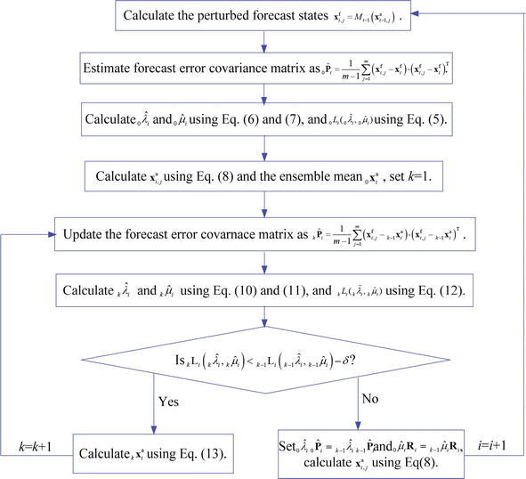
Figure 1.
Flowchart of EnKF with SLS inflation scheme.
which is a multiplicatively inflated sampling error covariance matrix plus an additive inflation matrix (see Appendix B for the proof).
2.3. Notes
2.3.1. Correctly specified observational error covariance matrix
If the observational error covariance matrix Ri is correctly known, then its adjustment is no longer required. In this case, the inflation factor λ̂ki can be estimated by minimizing the following objective function
E15
This leads to a simpler estimate
E16
2.3.2. Validation statistics
In any toy model, the “true” state xit is known by experimental design. In this case, the root-mean-square error (RMSE) of the analysis state can be used to evaluate the accuracy of the assimilation results. The RMSE at i-th step is defined as
E17
where xika and xikt are the k-th components of the analysis state and true state at the i-th time step. In principle, a smaller RMSE indicates a better performance of the assimilation scheme.
Advertisement
3. Experiment on Lorenz 96 model
In this section, the EnKF with SLS inflation assimilation scheme is applied to a nonlinear dynamical system, which has properties relevant to realistic forecast problems: the Lorenz-96 model [39] with model error and a linear observational system. The performances of the assimilation schemes in Section 2 are evaluated through the following experiments.
3.1. Description of forecast and observational systems
The Lorenz-96 model [39] is a strongly nonlinear dynamical system with quadratic nonlinearity, which is governed by the equation.
E18
where k=1,2,⋯,K (K=40; hence, there are 40 variables). For Eq. (18) to be well-defined for all values of k, it is defined that X−1=XK−1,X0=XK,XK+1=X1. The dynamics of Eq. (18) are “atmosphere-like” in that the three terms on the right-hand side consist of a nonlinear advection-like term, a damping term, and an external forcing term respectively. These three terms can be thought of as some atmospheric quantity (e.g., zonal wind speed) distributed on a latitude circle. Therefore, the Lorenz-96 model has been widely used as a test bed to evaluate the performance of assimilation schemes in many studies [30].
The true state is derived by a fourth-order Runge–Kutta time integration scheme [40]. The time step for generating the numerical solution was set at 0.05 nondimensional units, which is roughly equivalent to 6 hours in real time, assuming that the characteristic time-scale of the dissipation in the atmosphere is 5 days [39]. The forcing term was set as F = 8, so that the leading Lyapunov exponent implies an error-doubling time of approximately 8 time steps, and the fractal dimension of the attractor was 27.1 [41]. The initial value was chosen to be Xk=F when k≠20 and X20=1.001F.
In this study, the synthetic observations were assumed to be generated by adding random noises that were multivariate-normally distributed with mean zero and covariance matrix Ri to the true states. The frequency was four time steps, which can be used to mimic daily observations in practical problems, such as satellite data. The observation errors were assumed to be spatially correlated, which is common in applications involving remote sensing and radiance data. The variance of the observation at each grid point was set to σo2=1, and the covariance of the observations between the j-th and k-th grid points was as follows:
E19
Since it can deal with spatially correlated observational errors, the scheme may potentially be applied for assimilating remote sensing observations and radiances data.
The model errors by changing the forcing term are added in the forecast model because it is inevitable in real dynamic systems. Thus, different values of F are chose in the assimilation schemes while retaining F = 8 when generating the “true” state. The observations are simulated every four time steps analogizing 1 day in realistic problem for 2000 steps to ensure robust results. The ensemble size is used as 30. The pre-determined threshold δ to control the convergence of Eq. (12) is set to be 1, because the values of objective functions are in the order of 105. In most cases of the following experiment, the objective functions converge after 3–4 iterations, and the estimated analysis states also converge.
3.2. Comparison of assimilation schemes
In Section 2.1, the EnKF assimilation scheme with SLS error covariance matrix inflation is outlined. In Section 2.2, the improved EnKF assimilation scheme with the SLS error covariance matrix inflation and the new structure of the forecast error covariance matrix are summarized. In the following, the influences of these estimation methods on EnKF data assimilation schemes are assessed using Lorenz-96 model.
Lorenz-96 model is a forced dissipative model with a parameter F that controls the strength of the forcing (Eq. (18)). The model behaviors are quite different with different values of F, and chaotic systems are produced with integer values of F larger than 3. Therefore, several values of F are used to simulate a wide range of model errors. In all cases, the true states were generated by a model with F = 8. These observations were then assimilated into models with F = 4, 5, …, 12.
3.2.1. Correctly specified observational error covariance matrix
Suppose the observational error covariance matrix Ri is correctly specified, the inflation adjustment on P̂i is taken in each assimilation cycle and estimate the inflation factors λi by the methods described in Section 2.1. Then, the adaptive assimilation schemes with the new structure of the forecast error covariance matrix proposed in Section 2.2 are conducted.
Figure 2 shows the time-mean analysis RMSE of the two assimilation schemes averaged over 2000 time steps, as a function of F. Overall, the analysis RMSE of the two assimilation schemes gradually grows as increasing model error. When F is near the true value 8, the two assimilation schemes have almost indistinguishable values of the analysis RMSE. However, when F becomes increasingly distant from 8, the analysis RMSE of the assimilation scheme with the new structure of the forecast error covariance matrix becomes progressively smaller than that of the assimilation scheme with the forecast error covariance matrix inflation only.

Figure 2.
Time-mean values of the analysis RMSE as a function of forcing F when observational errors are spatially correlated and their covariance matrix is correctly specified, by using 3 EnKF schemes. 1) SLS only (solid line, described in Section 2.1); 2) SLS and new structure (dashed line, described in Section 2.2); and 3) SLS and true ensemble forecast error (dotted line, described in Section 5).
For the Lorenz-96 model with large error (such as, the case with F = 12), the time-mean analysis RMSE of the two assimilation schemes is listed in Table 1, as well as the time-mean values of the objective functions. The conventional EnKF assimilation scheme is also included for comparison. These results show clearly that our two schemes have significantly smaller RMSE than the EnKF assimilation scheme. Moreover, the assimilation scheme with the new structure of the forecast error covariance matrix performs much better than assimilation scheme with forecast error covariance matrix inflation only.
| EnKF schemes | Time-mean RMSE | Time-mean L |
|---|---|---|
| Non-inflation | 5.65 | 2,298,754 |
| SLS | 1.89 | 148,468 |
| SLS and new structure | 1.22 | 38,125 |
| SLS and true ensemble forecast error | 0.48 | 19,652 |
Table 1.
The time-mean analysis RMSE and the time-mean objective function values in 4 EnKF schemes for Lorenz-96 model when observational errors are spatially correlated and their covariance matrix is correctly specified: (1) EnKF (non-inflation); (2) the SLS scheme in Section 2.1 (SLS); (3) the SLS scheme in Section 2.2 (SLS and new structure); (4) the SLS scheme in the discussion (SLS and true ensemble forecast error). The forcing term F = 12.
3.2.2. Incorrectly specified observational error covariance matrix
In this section, the observational error covariance matrix is supposed to be correct only up to a constant factor. The factor is estimated using different estimation methods, and the corresponding assimilation results are evaluated.
The observational error covariance matrix Ri is set as four times of the true matrix and introduces another factor μi to adjust Ri. The assimilation schemes are conducted in two cases: (1) inflate the forecast and observational error covariance matrices only (Section 2.1); (2) inflate the forecast and observational error covariance matrices and use the new structure of the forecast error covariance matrix (Section 2.2). Again, the forcing term F takes values 4, 5, …, 12 when assimilating observations, but F = 8 is used when generating the true states in all cases.
Figure 3 shows the time-mean analysis RMSE of the two cases averaged over 2000 time steps, as a function of forcing term. Generally speaking, the analysis RMSE of the two cases gradually grows as the increasing the model error. However, the analysis RMSE generated by using new structure of the forecast error covariance matrix (cases 2) is smaller than those by using the error covariance matrices inflation technique only (cases 1).
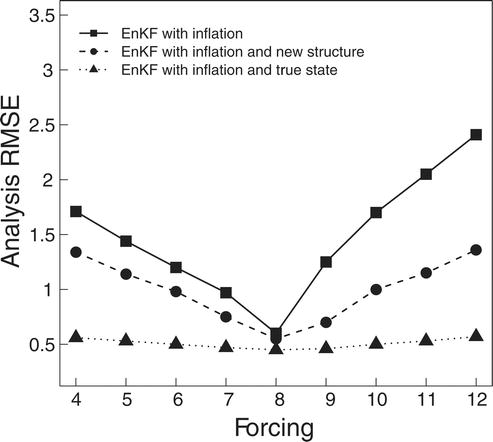
Figure 3.
Time-mean values of the analysis RMSE as a function of forcing F when observational errors are spatially correlated and their covariance matrix is incorrectly specified, by using 3 EnKF schemes. 1) SLS only (solid line); 2) SLS and new structure (dashed line); and 3) SLS and true ensemble forecast error (dotted line).
For the Lorenz-96 model with forcing term F = 12, the time-mean analysis RMSE of the two cases is listed in Table 2, along with the time-mean values of the objective functions. These results clearly show that when the observational error covariance matrix is incorrectly specified, the assimilation result is much better if the new structure of the forecast error covariance matrix is used (cases 2).
| EnKF schemes | Ensemble size 30 | Ensemble size 20 | ||
|---|---|---|---|---|
| Time-mean RMSE | Time-mean L | Time-mean RMSE | Time-mean L | |
| SLS | 2.43 | 1,426,541 | 3.51 | 1,492,685 |
| SLS and new structure | 1.35 | 41,326 | 1.45 | 95,685 |
| SLS and true ensemble forecast error | 0.58 | 21,585 | 0.60 | 21,355 |
Table 2.
The time-mean analysis RMSE and the time-mean objective function values in EnKF schemes for Lorenz-96 model when observational errors are spatially correlated and their covariance matrix is incorrectly specified: (1) SLS; (2) SLS and new structure; (4) SLS and true ensemble forecast error. The forcing term F = 12.
The estimated μ̂i over 2000 time steps in the two cases of using the new structure of the forecast error covariance matrix (cases 2) are plotted in Figure 4. It can be seen that the time-mean value of estimated μ̂i is 0.45, which is very close to the reciprocal of the constant that is multiplied to the observational error covariance matrix (0.25).

Figure 4.
The times series of estimated μ̂i when observational error covariance matrix is incorrectly specified.
To further investigate the effect of ensemble size on the assimilation result, Figure 3 is reproduced with the ensemble size 20. The results are shown in Figure 5, as well as in Table 2. Generally speaking, Figures 5 is quite similar to Figure 3 but with larger analysis error. This indicates that the smaller ensemble size can lead to the larger forecast error and analysis error. The analysis is also repeated with the ensemble size 10. However in this case, both the inflation and new structure are not effective. This could be due to that the ensemble size 10 is too small to generate robust covariance estimation.

Figure 5.
Similar to Figure 3, but ensemble size is 20.
Advertisement
4. Discussion and conclusions
It is well-known that accurately estimating the error covariance matrix is one of the most key steps in any ensemble-based data assimilation. In EnKF assimilation scheme, the forecast error covariance matrix is initially estimated as the sampling covariance matrix of the ensemble forecast states. But due to limited ensemble size and model error, the forecast error covariance matrix is usually an underestimation, which may lead to the divergence of the filter. Therefore, the initially estimated forecast error covariance matrix is multiplied by an inflation factor λi, and the SLS estimation is proposed to estimate this factor.
In fact, the true forecast error should be represented as the ensemble forecast states minus the true state. However, since in real problems, the true state is not available, the ensemble mean of the forecast states is used instead. Consequently, the forecast error covariance matrix is initially represented as the sampling covariance matrix of the ensemble forecast states. However, for the model with large error, the ensemble mean of the forecast states may be far from the true state. In this case, the estimated forecast error covariance matrix will also remain far from the truth, no matter which inflation technique is used.
To verify this point, a number of EnKF assimilation schemes with necessary error covariance matrix inflation are applied to the Lorenz-96 model but with the forecast state xif in the forecast error covariance matrix (Eq. (4)) substituted by the true state xit. The corresponding RMSE are shown in Figures 2–5 and Tables 1 and 2. All the figures and tables show that the analysis RMSE is significantly reduced.
However, since the true state xit is unknown, the analysis state xia is used to replace the forecast state xif, because xia is closer to xit than xif. To achieve this goal, a new structure of the forecast error covariance matrix and an adaptive procedure for estimating the new structure are proposed here to iteratively improve the estimation. As shown in this chapter, the RMSE of the corresponding analysis states are indeed smaller than those of the EnKF assimilation scheme with the error covariance matrix inflation only. For instance, in the experiment in Section 3.1, when the error covariance matrix inflation technique is applied, the RMSE is 1.89 which is much smaller than that for the original EnKF. When the new structure of the forecast error covariance matrix is used in addition to the inflation, the RMSE is reduced to 1.22 (see Table 1).
In the realistic problems, the observational error covariance matrix is not always correctly known, and hence it also needs to be adjusted too. Another factor μi is introduced to adjust the observational error covariance matrix in this chapter, which can be estimated simultaneously with λi by minimizing the second-order least squares function of the squared observation-minus-forecast residual.
The second-order least squares function of the squared observation-minus-forecast residual can be a good objective function to quantify the goodness of fit of the error covariance matrix. The SLS method proposed in this chapter can be used to estimate the factors for adjusting both the forecast and observational error covariance matrices, while the first order method can only estimate the inflation factor of the forecast error covariance matrix. The SLS can also provide a criterion for stopping the iteration in the adaptive estimation procedure when the new structure of the forecast error covariance matrix is used. This is important for preventing the proposed forecast error covariance matrix to depart from the truth in the iteration. In most cases in this study, the minimization algorithms converge after several iterations, and the objective function decreases sharply. On the other hand, the improved forecast error covariance matrix indeed leads to the improvement of analysis state. In fact, as shown in Tables 1—2, a small objective function value always corresponds to a small RMSE of the analysis state.
The difference of the EnKF assimilation scheme with SLS inflation is compared to that with maximum likelihood estimation (MLE) inflation [21]. Generally speaking, the RMSE of the analysis state derived using the MLE inflation scheme is a little smaller than that derived using the SLS inflation scheme only but is larger than that derived using the SLS inflation with the new structure of forecast error covariance matrix. For instance, for Lorenz-96 model with forcing term F = 12, the RMSE is 1.69 for MLE inflation, 1.89 for SLS inflation only, and 1.22 for SLS inflation and new structure (Table 1). Whether this is a general rule or not is still unclear and is subject to further investigation. However, in MLE inflation scheme, the objective function is nonlinear and especially involves the determinant of the observation-minus-forecast residual’s covariance matrix, which is quite computationally expensive. The SLS objective function proposed in this chapter is quadratic, so its minimizer is analytic and can be easily calculated.
On the other hand, similar to other inflation schemes with single factor, this study also assumes the inflation factor to be constant in space. Apparently, this is not the case in many practical applications, especially for the cases that the observations are unevenly distributed. Persistently applying the same inflation values that are reasonably large to address problems in densely observed areas to all state variables can systematically overinflate the ensemble variances in sparsely observed areas [13, 26, 42]. Even when the adaptive procedure for estimating the error covariance matrix is applied, the problem may still exist in some extent. In the two case studies conducted here, the observational systems are relatively evenly distributed.
In the future study, we will investigate how to modify the adaptive procedure to suit the system with unevenly distributed observations. We also plan to apply our methodology to error covariance localization [43, 44] and to validate the proposed methodologies using more sophisticated dynamic and observational systems.
Advertisement
Acknowledgments
This work is supported by the National Natural Science Foundation of China (grant no. 91647202), the National Basic Research Program of China (grant no. 2015CB953703), the National Natural Science Foundation of China (grant no. 41405098) and the Fundamental Research Funds for the Central Universities. The authors gratefully acknowledge the anonymous reviewers for their constructive and relevant comments, which helped greatly in improving the quality of this manuscript. The authors are also grateful to the editors for their hard work and suggestions on this manuscript. Parts of this chapter are reproduced from the authors’ previous publications [29, 30].
Advertisement
The forecast error covariance matrix P̂i is inflated to λP̂i. The estimation of the inflation factors λ is based on the observation-minus-forecast residual
EA1
The covariance matrix of the random vector di can be expressed as a second-order regression equation [27]:
EA2
where E is the expectation operator and Ξ is the error matrix. The left-hand side of (A2) can be decomposed as
EA3
Since the forecast and observational errors are statistically independent, we have
EA4
EA5
From Eq. (2), yio−Hixit is the observational error at i-th time step, and hence
EA6
Further, since the forecast state xi,jf is treated as a random vector with the true state xit as its population mean,
EA7
Substituting Eqs (A3)–(A7) into Eq. (A2), we have
It follows that the second-order moment statistic of error Ξ can be expressed as
EA9
Therefore, λ can be estimated by minimizing objective function Liλ. Since Liλ is a quadratic function of λ with positive quadratic coefficients, the inflation factor can be easily expressed as
EA10
Similarly, if the amplitude of the observational error covariance matrix is not correct, we can adjust Ri to μiRi as well [21, 22]. Then, the objective function becomes
EA11
As a bivariate function of λ and μ, the first partial derivative with respect to the two parameters respectively are
EA12
and
EA13
Setting Eqs (A12)–(A13) to zero and solving them lead to
EA14
EA15
In fact,
EB1
Since xif is the ensemble mean forecast, we have
EB2
and similarly.
EB3
That is, the last two terms of Eq. (B1) vanish. Therefore, the proposed forecast error covariance matrix can be expressed as
EB4
References
- 1. Miller RN, Ghil M, Gauthiez F. Advanced data assimilation in strongly nonlinear dynamical systems. Journal of the Atmospheric Sciences. 1994;51:1037-1056
- 2. Ravazzani G et al. Potentialities of ensemble strategies for flood forecasting over the Milano urban area. Journal of Hydrology. 2016;539:237-253
- 3. Talagrand O. Assimilation of observations, an introduction. Journal of the Meteorological Society of Japan. 1997;75:191-209
- 4. Wang Y et al. Improving precipitation forecast with hybrid 3DVar and time-lagged ensembles in a heavy rainfall event. Atmospheric Research. 2017;183:1-16
- 5. Reichle RH. Data assimilation methods in the earth sciences. Advances in Water Resources. 2008;31:1411-1418
- 6. Yang SC, Kalnay E, Hunt B. Handling nonlinearity in an ensemble Kalman filter experiments with the three-variable Lorenz model. Monthly Weather Review. 2012;140:2628-2645
- 7. Sakov P, Oliver DS, Bertino L. An iterative EnKF for strongly nonlinear systems. Monthly Weather Review. 2012;140:1988-2004
- 8. Evensen G. Sequential data assimilation with a nonlinear quasi-geostrophic model using Monte Carlo methods to forecast error statistics. Journal of Geophysical Research. 1994;99:10143-10162
- 9. Burgers G, Leeuwen PJ, Evensen G. Analysis scheme in the ensemble kalman filter. Monthly Weather Review. 1998;126:1719-1724
- 10. Luo X, Hoteit I. Ensemble Kalman filtering with residual nudging: An extension to state estimation problems with nonlinear observation operators. Monthly Weather Review. 2014;142:3696-3712
- 11. Anderson JL, Anderson SL. A Monte Carlo implementation of the nonlinear fltering problem to produce ensemble assimilations and forecasts. Monthly Weather Review. 1999;127:2741-2758
- 12. Constantinescu EM et al. Ensemble-based chemical data assimilation I: General approach. Quarterly Journal of the Royal Meteorological Society. 2007;133:1229-1243
- 13. Hamill TM, Whitaker JS. Accounting for the error due to unresolved scales in ensemble data assimilation: A comparison of different approaches. Monthly Weather Review. 2005;133:3132-3147
- 14. Bai Y, Li X. Evolutionary algorithm-based error parameterization methods for data assimilation. Monthly Weather Review. 2011;139:2668-2685
- 15. Luo X, Hoteit I. Robust ensemble filtering and its relation to covariance inflation in the ensemble Kalman filter. Monthly Weather Review. 2011;139:3938-3953
- 16. Dee DP. On-line estimation of error covariance parameters for atmospheric data assimilation. Monthly Weather Review. 1995;123:1128-1145
- 17. Dee DP, Silva AM. Maximum-likelihood estimation of forecast and observation error covariance parameters part I: Methodology. Monthly Weather Review. 1999;127:1822-1834
- 18. Li H, Kalnay E, Miyoshi T. Simultaneous estimation of covariance inflatioin and observation errors within an ensemble Kalman filter. Quarterly Journal of the Royal Meteorological Society. 2009;135:523-533
- 19. Wang X, Bishop CH. A comparison of breeding and ensemble transform kalman filter ensemble forecast schemes. Journal of the Atmospheric Sciences. 2003;60:1140-1158
- 20. Miyoshi T. The Gaussian approach to adaptive covariance inflation and its implementation with the local ensemble transform Kalman filter. Monthly Weather Review. 2011;139:1519-1534
- 21. Liang X et al. Maximum likelihood estimation of inflation factors on error covariance matrices for ensemble Kalman filter assimilation. Quarterly Journal of the Royal Meteorological Society. 2012;138:263-273
- 22. Zheng X. An adaptive estimation of forecast error statistic for Kalman filtering data assimilation. Advances in Atmospheric Sciences. 2009;26:154-160
- 23. Zheng X et al. Using analysis state to construct forecast error covariance matrix in EnKF assimilation. Advances in Atmospheric Sciences. 2013;30:1303-1312
- 24. Wu G, Dan B, Zheng X. Soil moisture assimilation using a modified ensemble transform Kalman filter based on station observations in the Hai River basin. Advances in Meteorology. 2016
- 25. Anderson JL. An adaptive covariance inflation error correction algorithm for ensemble filters. Tellus. 2007;59A:210-224
- 26. Anderson JL. Spatially and temporally varying adaptive covariance inflation for ensemble filters. Tellus. 2009;61A:72-83
- 27. Wang L, Leblanc A. Second-order nonlinear least squares estimation. Annals of the Institute of Statistical Mathematics. 2008;60:883-900
- 28. Huang C, Wu G, Zheng X. A new estimation method of ensemble forecast error in ETKF assimilation with nonlinear observation operator. SOLA. 2017;13:63-68
- 29. Wu G et al. Improving the ensemble transform Kalman filter using a second-order Taylor approximation of the nonlinear observation operator. Nonlinear Processes in Geophysics. 2014;21:955-970
- 30. Wu G et al. A new structure for error covariance matrices and their adaptive estimation in EnKF assimilation. Quarterly Journal of the Royal Meteorological Society. 2013;139:795-804
- 31. Craven P, Wahba G. Smoothing noisy data with spline functions. Numerische Mathematik. 1979;31:377-403
- 32. Wahba G et al. Adaptive tuning of numerical weather prediction models randomized GCV in three- and four-dimensional data assimilation. Monthly Weather Review. 1995;123:3358-3369
- 33. Wu G, Zheng X. An estimate of the inflation factor and analysis sensitivity in the ensemble Kalman filter. Nonlinear Processes in Geophysics. 2017;24:329-341
- 34. Evensen G. The ensemble Kalman filter theoretical formulation and practical implementation. Ocean Dynamics. 2003;53:343-367
- 35. Ide K et al. Unified notation for data assimilation operational sequential and variational. Journal of the Meteorological Society of Japan. 1997;75:181-189
- 36. Houtekamer PL, Mitchell HL. A sequential ensemble Kalman filter for atmospheric data assimilation. Monthly Weather Review. 2001;129:123-137
- 37. Golub GH, Loan CFV. Matrix Computations. Baltimore: The Johns Hopkins University Press; 1996
- 38. Tippett MK et al. Notes and correspondence ensemble square root filter. Monthly Weather Review. 2003;131:1485-1490
- 39. Lorenz EN. Predictability a problem partly solved Paper presented at seminar on predictability. ECMWF: Reading UK; 1996
- 40. Butcher JC. Numerical methods for ordinary differential equations. JohnWiley & Sons. 2003:425
- 41. Lorenz EN, Emanuel KA. Optimal sites for supplementary weather observations simulation with a small model. Journal of the Atmospheric Sciences. 1998;55:399-414
- 42. Yang S-C, Kalnay E, Enomoto T. Ensemble singular vectors and their use as additive inflation in EnKF. Tellus A. 2015;67
- 43. Desroziers G, Arbogast E, Berre L. Improving spatial localization in 4DEnVar. Quarterly Journal of the Royal Meteorological Society. 2016;142:3171-3185
- 44. Kirchgessner P, Berger L, Gerstner AB. On the choice of an optimal localization radius in ensemble Kalman filter methods. Monthly Weather Review. 2014;142:2165-2175
Written By
Guocan Wu and Xiaogu Zheng
Submitted: August 14th, 2017 Reviewed: October 26th, 2017 Published: December 20th, 2017
© 2017 The Author(s). Licensee IntechOpen. This chapter is distributed under the terms of the Creative Commons Attribution 3.0 License, which permits unrestricted use, distribution, and reproduction in any medium, provided the original work is properly cited.
In probability theory and statistics, covariance is a measure of the joint variability of two random variables.[1] If the greater values of one variable mainly correspond with the greater values of the other variable, and the same holds for the lesser values (that is, the variables tend to show similar behavior), the covariance is positive.[2] In the opposite case, when the greater values of one variable mainly correspond to the fewer values of the other, (that is, the variables tend to show opposite behavior), the covariance is negative. The sign of the covariance, therefore, shows the tendency in the linear relationship between the variables. The magnitude of the covariance is the geometric mean of the variances that are in-common for the two random variables. The correlation coefficient normalizes the covariance by dividing by the geometric mean of the total variances for the two random variables.
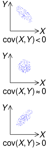
The sign of the covariance of two random variables X and Y
This article is about the degree to which random variables vary similarly. For other uses, see Covariance (disambiguation).
A distinction must be made between (1) the covariance of two random variables, which is a population parameter that can be seen as a property of the joint probability distribution, and (2) the sample covariance, which in addition to serving as a descriptor of the sample, also serves as an estimated value of the population parameter.
DefinitionEdit
For two jointly distributed real-valued random variables and with finite second moments, the covariance is defined as the expected value (or mean) of the product of their deviations from their individual expected values:[3][4]: p. 119
where is the expected value of , also known as the mean of . The covariance is also sometimes denoted or , in analogy to variance. By using the linearity property of expectations, this can be simplified to the expected value of their product minus the product of their expected values:
but this equation is susceptible to catastrophic cancellation (see the section on numerical computation below).
The units of measurement of the covariance are those of times those of . By contrast, correlation coefficients, which depend on the covariance, are a dimensionless measure of linear dependence. (In fact, correlation coefficients can simply be understood as a normalized version of covariance.)
Definition for complex random variablesEdit
The covariance between two complex random variables is defined as[4]: p. 119
Notice the complex conjugation of the second factor in the definition.
A related pseudo-covariance can also be defined.
Discrete random variablesEdit
If the (real) random variable pair can take on the values for , with equal probabilities , then the covariance can be equivalently written in terms of the means and as
It can also be equivalently expressed, without directly referring to the means, as[5]
More generally, if there are possible realizations of , namely but with possibly unequal probabilities for , then the covariance is
ExamplesEdit
Consider 3 independent random variables and two constants .
In the special case, and , the covariance between and , is just the variance of and the name covariance is entirely appropriate.
Geometric interpretation of the covariance example. Each cuboid is the axis-aligned bounding box of its point (x, y, f (x, y)), and the X and Y means (magenta point). The covariance is the sum of the volumes of the cuboids in the 1st and 3rd quadrants (red) minus those in the 2nd and 4th (blue).
Suppose that and have the following joint probability mass function,[6] in which the six central cells give the discrete joint probabilities of the six hypothetical realizations :
| x | |||||
|---|---|---|---|---|---|
| 5 | 6 | 7 | |||
| y | 8 | 0 | 0.4 | 0.1 | 0.5 |
| 9 | 0.3 | 0 | 0.2 | 0.5 | |
| 0.3 | 0.4 | 0.3 | 1 |
can take on three values (5, 6 and 7) while can take on two (8 and 9). Their means are and . Then,
PropertiesEdit
Covariance with itselfEdit
The variance is a special case of the covariance in which the two variables are identical (that is, in which one variable always takes the same value as the other):[4]: 121
Covariance of linear combinationsEdit
If , , , and are real-valued random variables and are real-valued constants, then the following facts are a consequence of the definition of covariance:
For a sequence of random variables in real-valued, and constants , we have
Hoeffding’s covariance identityEdit
A useful identity to compute the covariance between two random variables is the Hoeffding’s covariance identity:[7]
where is the joint cumulative distribution function of the random vector and are the marginals.
Uncorrelatedness and independenceEdit
Random variables whose covariance is zero are called uncorrelated.[4]: p. 121 Similarly, the components of random vectors whose covariance matrix is zero in every entry outside the main diagonal are also called uncorrelated.
If and are independent random variables, then their covariance is zero.[4]: p. 123 [8] This follows because under independence,
The converse, however, is not generally true. For example, let be uniformly distributed in and let . Clearly, and are not independent, but
In this case, the relationship between and is non-linear, while correlation and covariance are measures of linear dependence between two random variables. This example shows that if two random variables are uncorrelated, that does not in general imply that they are independent. However, if two variables are jointly normally distributed (but not if they are merely individually normally distributed), uncorrelatedness does imply independence.
Relationship to inner productsEdit
Many of the properties of covariance can be extracted elegantly by observing that it satisfies similar properties to those of an inner product:
- bilinear: for constants and and random variables
- symmetric:
- positive semi-definite: for all random variables , and implies that is constant almost surely.
In fact these properties imply that the covariance defines an inner product over the quotient vector space obtained by taking the subspace of random variables with finite second moment and identifying any two that differ by a constant. (This identification turns the positive semi-definiteness above into positive definiteness.) That quotient vector space is isomorphic to the subspace of random variables with finite second moment and mean zero; on that subspace, the covariance is exactly the L2 inner product of real-valued functions on the sample space.
As a result, for random variables with finite variance, the inequality
holds via the Cauchy–Schwarz inequality.
Proof: If , then it holds trivially. Otherwise, let random variable
Then we have
Calculating the sample covarianceEdit
The sample covariances among variables based on observations of each, drawn from an otherwise unobserved population, are given by the matrix with the entries
which is an estimate of the covariance between variable and variable .
The sample mean and the sample covariance matrix are unbiased estimates of the mean and the covariance matrix of the random vector , a vector whose jth element is one of the random variables. The reason the sample covariance matrix has in the denominator rather than is essentially that the population mean is not known and is replaced by the sample mean . If the population mean is known, the analogous unbiased estimate is given by
- .
GeneralizationsEdit
Auto-covariance matrix of real random vectorsEdit
For a vector of jointly distributed random variables with finite second moments, its auto-covariance matrix (also known as the variance–covariance matrix or simply the covariance matrix) (also denoted by or ) is defined as[9]: p.335
Let be a random vector with covariance matrix Σ, and let A be a matrix that can act on on the left. The covariance matrix of the matrix-vector product A X is:
This is a direct result of the linearity of expectation and is useful
when applying a linear transformation, such as a whitening transformation, to a vector.
Cross-covariance matrix of real random vectorsEdit
For real random vectors and , the cross-covariance matrix is equal to[9]: p.336
where is the transpose of the vector (or matrix) .
The -th element of this matrix is equal to the covariance between the i-th scalar component of and the j-th scalar component of . In particular, is the transpose of .
Cross-covariance sesquilinear form of random vectors in a real or complex Hilbert spaceEdit
More generally let and , be Hilbert spaces over or with anti linear in the first variable, and let be resp. valued random variables.
Then the covariance of and is the sesquilinear form on
(anti linear in the first variable) given by
Numerical computationEdit
When , the equation is prone to catastrophic cancellation if and are not computed exactly and thus should be avoided in computer programs when the data has not been centered before.[10] Numerically stable algorithms should be preferred in this case.[11]
Edit
The covariance is sometimes called a measure of «linear dependence» between the two random variables. That does not mean the same thing as in the context of linear algebra (see linear dependence). When the covariance is normalized, one obtains the Pearson correlation coefficient, which gives the goodness of the fit for the best possible linear function describing the relation between the variables. In this sense covariance is a linear gauge of dependence.
ApplicationsEdit
In genetics and molecular biologyEdit
Covariance is an important measure in biology. Certain sequences of DNA are conserved more than others among species, and thus to study secondary and tertiary structures of proteins, or of RNA structures, sequences are compared in closely related species. If sequence changes are found or no changes at all are found in noncoding RNA (such as microRNA), sequences are found to be necessary for common structural motifs, such as an RNA loop. In genetics, covariance serves a basis for computation of Genetic Relationship Matrix (GRM) (aka kinship matrix), enabling inference on population structure from sample with no known close relatives as well as inference on estimation of heritability of complex traits.
In the theory of evolution and natural selection, the Price equation describes how a genetic trait changes in frequency over time. The equation uses a covariance between a trait and fitness, to give a mathematical description of evolution and natural selection. It provides a way to understand the effects that gene transmission and natural selection have on the proportion of genes within each new generation of a population.[12][13] The Price equation was derived by George R. Price, to re-derive W.D. Hamilton’s work on kin selection. Examples of the Price equation have been constructed for various evolutionary cases.
In financial economicsEdit
Covariances play a key role in financial economics, especially in modern portfolio theory and in the capital asset pricing model. Covariances among various assets’ returns are used to determine, under certain assumptions, the relative amounts of different assets that investors should (in a normative analysis) or are predicted to (in a positive analysis) choose to hold in a context of diversification.
In meteorological and oceanographic data assimilationEdit
The covariance matrix is important in estimating the initial conditions required for running weather forecast models, a procedure known as data assimilation. The ‘forecast error covariance matrix’ is typically constructed between perturbations around a mean state (either a climatological or ensemble mean). The ‘observation error covariance matrix’ is constructed to represent the magnitude of combined observational errors (on the diagonal) and the correlated errors between measurements (off the diagonal). This is an example of its widespread application to Kalman filtering and more general state estimation for time-varying systems.
In micrometeorologyEdit
The eddy covariance technique is a key atmospherics measurement technique where the covariance between instantaneous deviation in vertical wind speed from the mean value and instantaneous deviation in gas concentration is the basis for calculating the vertical turbulent fluxes.
In signal processingEdit
The covariance matrix is used to capture the spectral variability of a signal.[14]
In statistics and image processingEdit
The covariance matrix is used in principal component analysis to reduce feature dimensionality in data preprocessing.
See alsoEdit
- Algorithms for calculating covariance
- Analysis of covariance
- Autocovariance
- Covariance function
- Covariance matrix
- Covariance operator
- Distance covariance, or Brownian covariance.
- Law of total covariance
- Propagation of uncertainty
ReferencesEdit
- ^ Rice, John (2007). Mathematical Statistics and Data Analysis. Belmont, CA: Brooks/Cole Cengage Learning. p. 138. ISBN 978-0534-39942-9.
- ^ Weisstein, Eric W. «Covariance». MathWorld.
- ^ Oxford Dictionary of Statistics, Oxford University Press, 2002, p. 104.
- ^ a b c d e Park,Kun Il (2018). Fundamentals of Probability and Stochastic Processes with Applications to Communications. Springer. ISBN 978-3-319-68074-3.
- ^ Yuli Zhang, Huaiyu Wu, Lei Cheng (June 2012). Some new deformation formulas about variance and covariance. Proceedings of 4th International Conference on Modelling, Identification and Control(ICMIC2012). pp. 987–992.
{{cite conference}}: CS1 maint: uses authors parameter (link) - ^ «Covariance of X and Y | STAT 414/415». The Pennsylvania State University. Archived from the original on August 17, 2017. Retrieved August 4, 2019.
- ^ Papoulis (1991). Probability, Random Variables and Stochastic Processes. McGraw-Hill.
- ^ Siegrist, Kyle. «Covariance and Correlation». University of Alabama in Huntsville. Retrieved Oct 3, 2022.
- ^ a b Gubner, John A. (2006). Probability and Random Processes for Electrical and Computer Engineers. Cambridge University Press. ISBN 978-0-521-86470-1.
- ^ Donald E. Knuth (1998). The Art of Computer Programming, volume 2: Seminumerical Algorithms, 3rd edn., p. 232. Boston: Addison-Wesley.
- ^ Schubert, Erich; Gertz, Michael (2018). «Numerically stable parallel computation of (co-)variance». Proceedings of the 30th International Conference on Scientific and Statistical Database Management – SSDBM ’18. Bozen-Bolzano, Italy: ACM Press: 1–12. doi:10.1145/3221269.3223036. ISBN 9781450365055. S2CID 49665540.
- ^ Price, George (1970). «Selection and covariance». Nature. 227 (5257): 520–521. Bibcode:1970Natur.227..520P. doi:10.1038/227520a0. PMID 5428476. S2CID 4264723.
- ^ Harman, Oren (2020). «When science mirrors life: on the origins of the Price equation». Phil. Trans. R. Soc. B. 375 (1797): 1–7. doi:10.1098/rstb.2019.0352. PMC 7133509. PMID 32146891. Retrieved 2020-05-15.
- ^ Sahidullah, Md.; Kinnunen, Tomi (March 2016). «Local spectral variability features for speaker verification». Digital Signal Processing. 50: 1–11. doi:10.1016/j.dsp.2015.10.011.