Improve Article
Save Article
Improve Article
Save Article
1. Flow Control :
It is an important function of the Data Link Layer. It refers to a set of procedures that tells the sender how much data it can transmit before waiting for acknowledgement from the receiver.
Purpose of Flow Control :
Any receiving device has a limited speed at which it can process incoming data and also a limited amount of memory to store incoming data. If the source is sending the data at a faster rate than the capacity of the receiver, there is a possibility of the receiver being swamped. The receiver will keep losing some of the frames simply because they are arriving too quickly and the buffer is also getting filled up.
This will generate waste frames on the network. Therefore, the receiving device must have some mechanism to inform the sender to send fewer frames or stop transmission temporarily. In this way, flow control will control the rate of frame transmission to a value that can be handled by the receiver.
Example – Stop & Wait Protocol
2. Error Control :
The error control function of data link layer detects the errors in transmitted frames and re-transmit all the erroneous frames.
Purpose of Error Control :
The function of the error control function of the data link layer helps in dealing with data frames that are damaged in transit, data frames lost in transit, and the acknowledgement frames that are lost in transmission. The method used for error control is called Automatic Repeat Request which is used for the noisy channel.
Example – Stop & Wait ARQ and Sliding Window ARQ
Difference between Flow Control and Error Control :
| S.NO. | Flow control | Error control |
|---|---|---|
| 1. | Flow control is meant only for the transmission of data from sender to receiver. | Error control is meant for the transmission of error free data from sender to receiver. |
| 2. | For Flow control there are two approaches : Feedback-based Flow Control and Rate-based Flow Control. | To detect error in data, the approaches are : Checksum, Cyclic Redundancy Check and Parity Checking. To correct error in data, the approaches are : Hamming code, Binary Convolution codes, Reed-Solomon code, Low-Density Parity Check codes. |
| 3. | It prevents the loss of data and avoid over running of receive buffers. | It is used to detect and correct the error occurred in the code. |
| 4. | Example of Flow Control techniques are : Stop&Wait Protocol and Sliding Window Protocol. | Example of Error Control techniques are : Stop&Wait ARQ and Sliding Window ARQ. |
Introduction[edit | edit source]
Data Link Layer is layer 2 in OSI model. It is responsible for communications between adjacent network nodes. It handles the data moving in and out across the physical layer. It also provides a well defined service to the network layer. Data link layer is divided into two sub layers. The Media Access Control (MAC) and Logical Link Control (LLC).
Data-Link layer ensures that an initial connection has been set up, divides output data into data frames, and handles the acknowledgements from a receiver that the data arrived successfully. It also ensures that incoming data has been received successfully by analyzing bit patterns at special places in the frames.
In the following sections data link layer’s functions- Error control and Flow control has been discussed. After that MAC layer is explained. Multiple access protocols are explained in the MAC layer section.
Error Control[edit | edit source]
Network is responsible for transmission of data from one device to another device. The end to end transfer of data from a transmitting application to a receiving application involves many steps, each subject to error. With the error control process, we can be confident that the transmitted and received data are identical. Data can be corrupted during transmission. For reliable communication, error must be detected and corrected.
Error control is the process of detecting and correcting both the bit level and packet level errors.
Types of Errors
Single Bit Error
The term single bit error means that only one bit of the data unit was changed from 1 to 0 and 0 to 1.
Burst Error
In term burst error means that two or more bits in the data unit were changed. Burst error is also called packet level error, where errors like packet loss, duplication, reordering.
Error Detection
Error detection is the process of detecting the error during the transmission between the sender and the receiver.
Types of error detection
- Parity checking
- Cyclic Redundancy Check (CRC)
- Checksum
Redundancy
Redundancy allows a receiver to check whether received data was corrupted during transmission. So that he can request a retransmission.
Redundancy is the concept of using extra bits for use in error detection. As shown in the figure sender adds redundant bits (R) to the data unit and sends to receiver, when receiver gets bits stream and passes through checking function. If no error then data portion of the data unit is accepted and redundant bits are discarded. otherwise asks for the retransmission.
Parity checking
Parity adds a single bit that indicates whether the number of 1 bits in the preceding data is even or odd. If a single bit is changed in transmission, the message will change parity and the error can be detected at this point.
Parity checking is not very robust, since if the number of bits changed is even, the check bit will be invalid and the error will not be detected.
- Single bit parity
- Two dimension parity
Moreover, parity does not indicate which bit contained the error, even when it can detect it. The data must be discarded entirely, and re-transmitted from scratch. On a noisy transmission medium a successful transmission could take a long time, or even never occur. Parity does have the advantage, however, that it’s about the best possible code that uses only a single bit of space.
Cyclic Redundancy Check
CRC is a very efficient redundancy checking technique. It is based on binary division of the data unit, the remainder of which (CRC) is added to the data unit and sent to the receiver. The Receiver divides data unit by the same divisor. If the remainder is zero then data unit is accepted and passed up the protocol stack, otherwise it is considered as having been corrupted in transit, and the packet is dropped.
Sequential steps in CRC are as follows.
Sender follows following steps.
- Data unit is composite by number of 0s, which is one less than the divisor.
- Then it is divided by the predefined divisor using binary division technique. The remainder is called CRC. CRC is appended to the data unit and is sent to the receiver.
Receiver follows following steps.
- When data unit arrives followed by the CRC it is divided by the same divisor which was used to find the CRC (remainder).
- If the remainder result in this division process is zero then it is error free data, otherwise it is corrupted.
Diagram shows how to CRC process works.
[a] sender CRC generator [b] receiver CRC checker
Checksum
Check sum is the third method for error detection mechanism. Checksum is used in the upper layers, while Parity checking and CRC is used in the physical layer. Checksum is also on the concept of redundancy.
In the checksum mechanism two operations to perform.
Checksum generator
Sender uses checksum generator mechanism. First data unit is divided into equal segments of n bits. Then all segments are added together using 1’s complement. Then it is complemented ones again. It becomes Checksum and sends along with data unit.
Exp:
If 16 bits 10001010 00100011 is to be sent to receiver.
So the checksum is added to the data unit and sends to the receiver.
Final data unit is 10001010 00100011 01010000.
Checksum checker
Receiver receives the data unit and divides into segments of equal size of segments. All segments are added using 1’s complement. The result is complemented once again. If the result is zero, data will be accepted, otherwise rejected.
Exp:
The final data is nonzero then it is rejected.
Error Correction
This type of error control allows a receiver to reconstruct the original information when it has been corrupted during transmission.
Hamming Code
It is a single bit error correction method using redundant bits.
In this method redundant bits are included with the original data. Now, the bits are arranged such that different incorrect bits produce different error results and the corrupt bit can be identified. Once the bit is identified, the receiver can reverse its value and correct the error.
Hamming code can be applied to any length of data unit and uses the relationships between the data and the redundancy bits.
Algorithm:
- Parity bits are positions at the power of two (2 r).
- Rest of the positions is filled by original data.
- Each parity bit will take care of its bits in the code.
- Final code will sends to the receiver.
In the above example we calculates the even parities for the various bit combinations. the value for the each combination is the value for the corresponding r(redundancy)bit.
r1 will take care of bit 1,3,5,7,9,11. and it is set based on the sum of even parity bit. the same method for rest of the parity bits.
If the error occurred at bit 7 which is changed from 1 to 0, then receiver recalculates the same sets of bits used by the sender. By this we can identify the perfect location of error occurrence. once the bit is identified the receiver can reverse its value and correct the error.
Flow Control[edit | edit source]
Flow Control is one important design issue for the Data Link Layer that controls the flow of data between sender and receiver.
In Communication, there is communication medium between sender and receiver. When Sender sends data to receiver then there can be problem in below case :
1) Sender sends data at higher rate and receive is too sluggish to support that data rate.
To solve the above problem, FLOW CONTROL is introduced in Data Link Layer. It also works on several higher layers. The main concept of Flow Control is to introduce EFFICIENCY in Computer Networks.
Approaches of Flow Control
- Feed back based Flow Control
- Rate based Flow Control
Feed back based Flow Control is used in Data Link Layer and Rate based Flow Control is used in Network Layer.
Feed back based Flow Control
In Feed back based Flow Control, Until sender receives feedback from the receiver, it will not send next data.
Types of Feedback based Flow Control
A. Stop-and-Wait Protocol
B. Sliding Window Protocol
- A One-Bit Sliding Window Protocol
- A Protocol Using Go Back N
- A Protocol Using Selective Repeat
A. A Simplex Stop-and-Wait Protocol
In this Protocol we have taken the following assumptions:
- It provides unidirectional flow of data from sender to receiver.
- The Communication channel is assumed to be error free.
In this Protocol the Sender simply sends data and waits for the acknowledgment from Receiver. That’s why it is called Stop-and-Wait Protocol.
This type is not so much efficient, but it is simplest way of Flow Control.
In this scheme we take Communication Channel error free, but if the Channel has some errors then receiver is not able to get the correct data from sender so it will not possible for sender to send the next data (because it will not get acknowledge from receiver). So it will end the communication, to solve this problem there are two new concepts were introduced.
- TIMER, if sender was not able to get acknowledgment in the particular time than, it sends the buffered data once again to receiver. When sender starts to send the data, it starts timer.
- SEQUENCE NUMBER, from this the sender sends the data with the specific sequence number so after receiving the data, receiver sends the data with that sequence number, and here at sender side it also expect the acknowledgment of the same sequence number.
This type of scheme is called Positive Acknowledgment with Retransmission (PAR).
B. Sliding Window Protocol
Problems Stop –wait protocol
In the last protocols sender must wait for either positive acknowledgment from receiver or for time out to send the next frame to receiver. So if the sender is ready to send the new data, it can not send. Sender is dependent on the receiver.
Previous protocols have only the flow of one sided, means only sender sends the data and receiver just acknowledge it, so the twice bandwidth is used.
To solve the above problems the Sliding Window Protocol was introduce.
In this, the sender and receiver both use buffer, it’s of same size, so there is no necessary to wait for the sender to send the second data, it can send one after one without wait of the receiver’s acknowledgment.
And it also solve the problem of uses of more bandwidth, because in this scheme both sender and receiver uses the channel to send the data and receiver just send the acknowledge with the data which it want to send to sender, so there is no special bandwidth is used for acknowledgment, so the bandwidth is saved, and this whole process is called PIGGYBACKING.
Types of Sliding Window Protocol
i. A One-Bit Sliding Window Protocol
ii. A Protocol Using Go Back N
iii. A Protocol Using Selective Repeat
i. A One-Bit Sliding Window Protocol
This protocol has buffer size of one bit, so only possibility for sender and receiver to send and receive packet is only 0 and 1. This protocol includes Sequence, Acknowledge, and Packet number.It uses full duplex channel so there is two possibilities:
- Sender first start sending the data and receiver start sending data after it receive the data.
- Receiver and sender both start sending packets simultaneously,
First case is simple and works perfectly, but there will be an error in the second one. That error can be like duplication of the packet, without any transmission error.
ii. A Protocol Using Go Back N
The problem with pipelining is if sender sending 10 packets, but the problem occurs in 8th one than it is needed to resend whole data. So the protocol called Go back N and Selective Repeat were introduced to solve this problem.In this protocol, there are two possibility at the receiver’s end, it may be with large window size or it may be with window size one.

The window size at the receiver end may be large or only of one. In the case of window size is one at the receiver, as we can see in the figure (a), if sender wants to send the packet from one to ten but suppose it has error in 2nd packet, so sender will start from zero, one, two, etc. here we assume that sender has the time out interval with 8. So the time out will occur after the 8 packets, up to that it will not wait for the acknowledgment. In this case at the receiver side the 2nd packet come with error, and other up to 8 were discarded by receiver. So in this case the loss of data is more.
Whether in the other case with the large window size at receiver end as we can see in the figure (b) if the 2nd packet comes with error than the receiver will accept the 3rd packet but it sends NAK of 2 to the sender and buffer the 3rd packet. Receiver do the same thing in 4th and 5th packet. When the sender receiver the NAK of 2nd packet it immediately send the 2nd packet to the receiver. After receiving the 2nd packet, receiver send the ACK of 5th one as saying that it received up to 5 packet. So there is no need to resend 3rd , 4th and 5th packet again, they are buffered in the receiver side.
iii. A Protocol Using Selective Repeat
Protocol using Go back N is good when the errors are rare, but if the line is poor, it wastes a lot of bandwidth on retransmitted frames. So to provide reliability, Selective repeat protocol was introduced. In this protocol sender starts it’s window size with 0 and grows to some predefined maximum number. Receiver’s window size is fixed and equal to the maximum number of sender’s window size. The receiver has a buffer reserved for each sequence number within its fixed window.
Whenever a frame arrives, its sequence number is checked by the function to see if it falls within the window, if so and if it has not already been received, it is accepted and stored. This action is taken whether it is not expected by the network layer.
Here the buffer size of sender and receiver is 7 and as we can see in the figure (a), the sender sends 7 frames to the receiver and starts timer. When a receiver gets the frames, it sends the ACK back to the sender and it passes the frames to the Network Layer. After doing this, receiver empties its buffer and increased sequence number and expects sequence number 7,0,1,2,3,4,5. But if the ACK is lost, the sender will not receive the ACK. So when the timer expires, the sender retransmits the original frames, 0 to 6 to the receiver. In this case the receiver accepts the frames 0 to 5 (which are duplicated) and send it to the network layer. In this case protocol fails.
To solve the problem of duplication, the buffer size of sender and receiver should be (MAX SEQ + 1)/2 that is half of the frames to be send. As we can see in fig(c ), the sender sends the frames from 0 to 3 as it’s window size is 4. Receiver accepts the frames and sends acknowledgment to the sender and passes the frames to the network layer and increases the expected sequence number from 4 to 7. If the ACK is lost than sender will send 0 to 3 to receiver again but receiver is expecting to 4 to 7, so it will not accept it. So this way the problem of duplication is solved.
MAC[edit | edit source]
The data link layer is divided into two sublayers: The Media Access Control (MAC) layer and the Logical Link Control (LLC) layer. The MAC sublayer controls how a computer on the network gains access to the data and permission to transmit it. The LLC layer controls frame synchronization, flow control and error checking.
Mac Layer is one of the sublayers that makeup the datalink layer of the OSI reference Model.
MAC layer is responsible for moving packets from one Network Interface card NIC to another across the shared channel
The MAC sublayer uses MAC protocols to ensure that signals sent from different stations across the same channel don’t collide.
Different protocols are used for different shared networks, such as Ethernets, Token Rings, Token Buses, and WANs.
1. ALOHA
ALOHA is a simple communication scheme in which each source in a network sends its data whenever there is a frame to send without checking to see if any other station is active. After sending the frame each station waits for implicit or explicit acknowledgment. If the frame successfully reaches the destination, next frame is sent. And if the frame fails to be received at the destination it is sent again.
Pure ALOHA
ALOHA is the simplest technique in multiple accesses. Basic idea of this mechanism is a user can transmit the data whenever they want. If data is successfully transmitted then there isn’t any problem. But if collision occurs than the station will transmit again. Sender can detect the collision if it doesn’t receive the acknowledgment from the receiver.
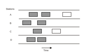
![Here packets sent at time t0 will collide with other packets sent in the time interval [t0-1, t0+1].](https://upload.wikimedia.org/wikipedia/commons/thumb/c/c2/Pure_ALOHA.svg/300px-Pure_ALOHA.svg.png)
In ALOHA Collision probability is quite high. ALOHA is suitable for the network where there is a less traffic. Theoretically it is proved that maximum throughput for ALOHA is 18%.
                     P (success by given node) = P(node transmits) . P(no other node transmits in [t0-1,t0] . P(no other node transmits in [t0,t0 +1]
                                               = p . (1-p)N-1 . (1-p)N-1
                 P (success by any of N nodes) = N . p . (1-p) N-1 . (1-p)N-1
                                               … Choosing optimum p as N -->  infinity...
                                               = 1 / (2e) = .18
                                               =18%
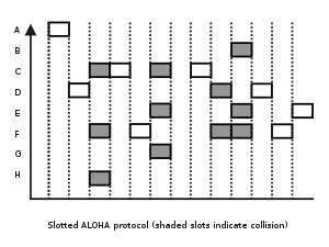
Slotted ALOHA
In ALOHA a newly emitted packet can collide with a packet in progress. If all packets are of the same length and take L time units to transmit, then it is easy to see that a packet collides with any other packet transmitted in a time window of length 2L.
If this time window is decreased somehow, than number of collisions decreases and the throughput increase. This mechanism is used in slotted ALOHA or S-ALOHA. Time is divided into equal slots of Length L. When a station wants to send a packet it will wait till the beginning of the next time slot.
Advantages of slotted ALOHA:
- single active node can continuously transmit at full rate of channel
- highly decentralized: only slots in nodes need to be in sync
- simple
Disadvantages of slotted ALOHA:
- collisions, wasting slots
- idle slots
- clock synchronization
Efficiency of Slotted ALOHA:
- Suppose there are N nodes with many frames to send. The probability of sending frames of each node into the slot is p.
- Probability that node 1 has a success in getting the slot is p.(1-p)N-1
- Probability that every node has a success is N.p.(1-p)N-1
- For max efficiency with N nodes, find p* that maximizes Np(1-p)N-1
- For many nodes, take limit of Np*(1-p*)N-1 as N goes to infinity, gives 1/e = .37
The clear advantage of slotted ALOHA is higher throughput. But introduces complexity in the stations and bandwidth overhead because of the need for time synchronization.
2. Carrier Sense Multiple Access protocols (CSMA)
With slotted ALOHA, the best channel utilization that can be achieved is 1/e. Several protocols are developed for improving the performance.
Protocols that listen for a carrier and act accordingly are called carrier sense protocols. Carrier sensing allows the station to detect whether the medium is currently being used. Schemes that use a carrier sense circuits are classed together as carrier sense multiple access or CSMA schemes. There are two variants of CSMA. CSMA/CD and
CSMA/CA
The simplest CSMA scheme is for a station to sense the medium, sending packets immediately if the medium is idle. If the station waits for the medium to become idle it is called persistent otherwise it is called non persistent.
a. Persistent
When a station has the data to send, it first listens the channel to check if anyone else is transmitting data or not. If it senses the channel idle, station starts transmitting the data. If it senses the channel busy it waits until the channel is idle. When a station detects a channel idle, it transmits its frame with probability P. That’s why this protocol is called p-persistent CSMA. This protocol applies to slotted channels. When a station finds the channel idle, if it transmits the fame with probability 1, that this protocol is known as 1 -persistent. 1 -persistent protocol is the most aggressive protocol.
b. Non-Persistent
Non persistent CSMA is less aggressive compared to P persistent protocol. In this protocol, before sending the data, the station senses the channel and if the channel is idle it starts transmitting the data. But if the channel is busy, the station does not continuously sense it but instead of that it waits for random amount of time and repeats the algorithm. Here the algorithm leads to better channel utilization but also results in longer delay compared to 1 –persistent.
CSMA/CD
Carrier Sense Multiple Access/Collision Detection a technique for multiple access protocols. If no transmission is taking place at the time, the particular station can transmit. If two stations attempt to transmit simultaneously, this causes a collision, which is detected by all participating stations. After a random time interval, the stations that collided attempt to transmit again. If another collision occurs, the time intervals from which the random waiting time is selected are increased step by step. This is known as exponential back off.
Exponential back off Algorithm
- Adaptor gets datagram and creates frame
- If adapter senses channel idle (9.6 microsecond), it starts to transmit frame. If it senses channel busy, waits until channel idle and then transmits
- If adapter transmits entire frame without detecting another transmission, the adapter is done with frame!
- If adapter detects another transmission while transmitting, aborts and sends jam signal
- After aborting, adapter enters exponential backoff: after the mth collision, adapter chooses a K at random from {0,1,2,…,2m-1}. Adapter waits K*512 bit times (i.e. slot) and returns to Step 2
- After 10th retry, random number stops at 1023. After 16th retry, system stops retry.
CSMA/CA
CSMA/CA is Carrier Sense Multiple Access/Collision Avoidance. In this multiple access protocol, station senses the medium before transmitting the frame. This protocol has been developed to improve the performance of CSMA. CASMA/CA is used in 802.11 based wireless LANs. In wireless LANs it is not possible to listen to the medium while transmitting. So collision detection is not possible.
In CSMA/CA, when the station detects collision, it waits for the random amount of time. Then before transmitting the packet, it listens to the medium. If station senses the medium idle, it starts transmitting the packet. If it detects the medium busy, it waits for the channel to become idle.

When A wants to transmit a packet to B, first it sends RTS (Request to Send) packet of 30 bytes to B with length L. If B is idle, it sends its response to A with CTS packet (Clear to Send). Here whoever listens to the CTS packet remains silent for duration of L.
When A receives CTS, it sends data of L length to B.
There are several issues in this protocol
- Hidden Station Problem
- Exposed Station Problem
1. Hidden Station Problem (Figure a)
When a station sends the packet to another station/receiver, some other station which is not in sender’s range may start sending the packet to the same receiver. That will create collision of packets. This problem is explained more specifically below.
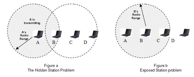
Suppose A is sending a packet to B. Now at the same time D also wants to send the packet to B. Here D does not hear A.
So D will also send its packets to B. SO collision will occur.
2. Exposed Station Problem (Figure b)
When A is sending the packet, C will also hear. So if station wants to send the packet D, still it won’t send. This will reduce the efficiency of the protocol.
This problem is called Exposed Station problem.
To deal with these problems 802.11 supports two kinds of operations.
- DCF (Distributed Coordination Function)
- PCF (Point Coordinated Function)
DCF
DCF does not use and central control. It uses CSMA/CA protocol. It uses physical channel sensing and virtual channel sensing. Here when a station wants to send packets, first it senses the channel. If the channel is idle, immediately starts transmitting. While transmitting, it does not sense the channel, but it emits its entire frame. This frame can be destroyed at the receiver side if receiver has started transmitting. In this case, if collision occurs, the colliding stations wait for random amount of time using the binary exponential back off algorithm and tries again letter.
Virtual sensing is explained in the figure given below.
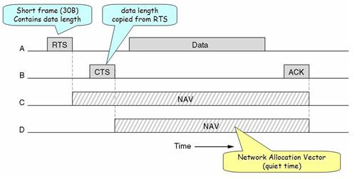
Here, A wants to send a packet to B. Station C is within A’s Range. Station D is within B’s range but not A’s range.
When A wants to send a packet to B, first it sends the RTS (30 bytes) packet to B, asking for the permission to send the packet. In the response, if B wants to grant the permission, it will send the CTS packet to A giving permission to A for sending the packet. When A receives its frame it starts ACK timer. When the frame is successfully transmitted, B sends ACK frame. Here if A’s ACK time expires before receiving B’s ACK frame, the whole process will run again.
Here for the stations C and D, when station A sends RTS to station B, RTS will also be received by C. By viewing the information provided in RTS, C will realize that some on is sending the packet and also how long the sequence will take, including the final ACK. So C will assert a kind of virtual channel busy by itself, (indicated by NAV (network Allocation Vector) in the figure above).remain silent for the particular amount of time. Station D will not receive RTS, but it will receive CTS from B. So B will also assert the NAV signal for itself.
If the channel is too noisy, when A send the frame to B and a frame is too large then there are more possibilities of the frame getting damaged and so the frame will be retransmitted. C and D, both stations will also remain silent until the whole frame is transmitted successfully. To deal with this problem of noisy channels, 802.11 allows the frame to be fragmented into smaller fragments. Once the channel has been acquired using CTS and RTS, multiple segments can be sent in a row. Sequence of segments is called a fragmentation burst. Fragmentation increases the throughput by restricting retransmissions to the bad fragments rather than the entire frame.

PCF
PCF mechanism uses base station to control all activity in its cell. Base station polls the other station asking them if they have any frame to send. In PCF, as it is centralized, no collision will occur.
In polling mechanism, the base station broadcasts a beacon frame periodically (10 to 100 times per second). Beacon frame contains system parameters such as hopping sequences, dwell times, clock synchronization etc. It also invites new station to sign up.
All signed up stations are guaranteed to get a certain fraction of the bandwidth. So in PCF quality of service is guaranteed.
All implementations must support DCF but PCF is optional. PCF and DCF can coexist within one sell. Distributed control and Centralized control, both can operate at the same time using interframe time interval. There are four interval defined. This four intervals are shown in the figure given below.

- SIFS — Short InterFrame Spacing
- PIFS – PCF InterFrame Spacing
- DIFS – DCF InterFrame Spacing
- EIFS – Extended Inter Frame Spacing
More about this has been explained in section 3 of Data Link Layer.
Taking Turns MAC protocols
Polling
In Polling, master node invites slave nodes to transmit in nodes.
Single point of failure (master node failure), polling overhead, latency are the concerns in polling.
Bit map Reservation
In Bit map reservation, stations reserves contention slots in advance.
Polling overhead and latency are the concerns in this protocol.

Token Passing
In this protocol, token is passed from one node to next sequentially. Single point of failure (token), token overhead, latency are the concerns in token passing.

Problems[edit | edit source]
- Explain hidden station and exposed station problem.
- Explain Binary Exponential Backoff Algorithm.
- Two CSMA/C stations are trying to transmit long files. After each frame is sent, they contend for the channel using binary exponential backoff algorithm. What is the probability that the connection ends on round k?
- In CRC , if th data unit is 101100 the divisor 1010 and the reminder is 110 what is the dividend at the receiver? (Ans: )
Further reading[edit | edit source]
- Serial Programming:Error Correction Methods
 Flow control and Error control are the control mechanism at data link layer and transport layer. Whenever the sends the data to the receiver these two mechanisms helps in proper delivering of the reliable data to the receiver. The main difference between the flow control and error control is that the flow control observes the proper flow of the data from sender to receiver, on the other hand, the error control observes that the data delivered to the receiver is error free and reliable.
Let’s study the difference between Flow control and Error control with a comparison chart.
Content: Flow Control Vs Error Control
- Comparison Chart
- Definition
- Key Differences
- Conclusion
Comparison Chart
| Basis for Comparison | Flow Control | Error Control |
|---|---|---|
| Basic | Flow control is meant for the proper transmission of the data from sender to the receiver. | Error control is meant for delivering the error-free data to the receiver. |
| Approach | Feedback-based flow control and rate-based flow control are the approaches to achieve the proper flow control. | Parity checking, Cyclic Redundancy Code (CRC) and checksum are the approaches to detect the error in data. Hamming code, Binary Convolution codes, Reed-Solomon code, Low-Density Parity Check codes are the approaches to correct the error in data. |
| Impact | avoid overrunning of receivers buffer and prevents the data loss. | Detects and correct the error occurred in the data. |
Definition of Flow Control
The flow control is a design issue at data link layer and transport layer. A sender sends the data frames faster then the receiver can accept. The reason can be that a sender is running on a powerful machine. In this case, even the data is received without any error; the receiver is unable to receive the frame at this speed and loose some frames.
There are two control methods to prevent the loss of frames they are feedback-based flow control and rate-based flow control.
Feedback-based control
In feedback-based control whenever the sender sends the data to the receiver, the receiver then sends the information back to the sender and permits the sender to send more data or inform the sender about how the receiver is doing. The protocols of feedback-based control are sliding window protocol, stop-and-wait protocol.
Rate-based flow control
In rate-based flow control, when a sender transmits the data faster to the receiver and receiver is unable to receive the data at that speed, then the built-in mechanism in the protocol will limit the rate at which data is being transmitted by the sender without any feedback from the receiver.
Definition of Error Control
Error Control is the issue that occurs at data link layer and transport level as well. Error Control is a mechanism for detecting and correcting the error occurred in frames that are delivered from sender to the receiver. The error occurred in the frame may be a single bit error or burst error. Single bit error is the error that occurs only in the one-bit data unit of the frame, where 1 is changed to 0 or 0 is changed to 1.
In burst error is the case when more than one bit in the frame is changed; it also refers to the packet level error. In burst error, the error like packet loss, duplication of the frame, loss of acknowledgment packet, etc. can also occur.The methods to detect the error in the frame are parity checking, cyclic redundancy code (CRC) and checksum.
Parity Checking
In parity checking, a single bit is added to the frame which indicates whether the number of ‘1’ bit contained in the frame are even or odd. During transmission, if a single bit gets changed the parity bit also get change which reflects the error in the frame. But the parity checking method is not reliable as if the even number of bits are changed then the parity bit will not reflect any error in the frame. However, it is best for single bit error.
Cyclic Redundancy Code (CRC)
In Cyclic Redundancy Code the data undergoes a binary division whatever the remainder is obtained is attached with the data and send to the receiver. The receiver then divides the obtained data with the same divisor as with which the sender divided the data. If the remainder obtained is zero then the data is accepted. Else the data is rejected, and the sender needs to retransmit the data again.
Checksum
In checksum method, the data to be send is divided into equal fragments each fragment containing n bits. All the fragments are added using 1’s complement. The result is complemented once again, and now the obtained series of bits is called checksum which is attached with the original data to be send and send to the receiver.
When the receiver receives the data, it also divides the data in equal fragment then add all the fragment using 1’s complement; the result is again complemented. If the result comes out to be zero then the data is accepted else it is rejected, and the sender has to retransmit the data.
The error obtained in the data can be corrected using methods they are Hamming code, Binary Convolution codes, Reed-Solomon code, Low-Density Parity Check codes.
- Flow control is to monitor the proper transmission of data from sender to receiver. On the other hand, Error Control monitors the error-free delivery of data from sender to receiver.
- Flow control can be achieved by the Feedback-based flow control and rate-based flow control approach whereas, to detect the error the approaches used are Parity checking, Cyclic Redundancy Code (CRC) and checksum and to correct the error the approaches used are Hamming code, Binary Convolution codes, Reed-Solomon code, Low-Density Parity Check codes.
- Flow control prevents the receivers buffer from overrunning and also prevents the loss of data. On the other hand, Error control detects and corrects error occurred in the data.
Conclusion
Both the control mechanism i.e. Flow control and Error control are the unavoidable mechanism for delivering a complete and reliable data.
In this tutorial, we will be covering the concept of Flow and Error Control in the Data Link layer.
Flow control and Error control are the two main responsibilities of the Data link layer. Let us understand what these two terms specify. For the node-to-node delivery of the data, the flow and error control are done at the data link layer.
Flow Control mainly coordinates with the amount of data that can be sent before receiving an acknowledgment from the receiver and it is one of the major duties of the data link layer.
-
For most of the protocols, flow control is a set of procedures that mainly tells the sender how much data the sender can send before it must wait for an acknowledgment from the receiver.
-
The data flow must not be allowed to overwhelm the receiver; because any receiving device has a very limited speed at which the device can process the incoming data and the limited amount of memory to store the incoming data.
-
The processing rate is slower than the transmission rate; due to this reason each receiving device has a block of memory that is commonly known as buffer, that is used to store the incoming data until this data will be processed. In case the buffer begins to fillup then the receiver must be able to tell the sender to halt the transmission until once again the receiver become able to receive.
Thus the flow control makes the sender; wait for the acknowledgment from the receiver before the continuation to send more data to the receiver.
Some of the common flow control techniques are: Stop-and-Wait and sliding window technique.
Error Control contains both error detection and error correction. It mainly allows the receiver to inform the sender about any damaged or lost frames during the transmission and then it coordinates with the retransmission of those frames by the sender.
The term Error control in the data link layer mainly refers to the methods of error detection and retransmission. Error control is mainly implemented in a simple way and that is whenever there is an error detected during the exchange, then specified frames are retransmitted and this process is also referred to as Automatic Repeat request(ARQ).
Protocols
The implementation of protocols is mainly implemented in the software by using one of the common programming languages. The classification of the protocols can be mainly done on the basis of where they are being used.
Protocols can be used for noiseless channels(that is error-free) and also used for noisy channels(that is error-creating). The protocols used for noiseless channels mainly cannot be used in real-life and are mainly used to serve as the basis for the protocols used for noisy channels.

All the above-given protocols are unidirectional in the sense that the data frames travel from one node i.e Sender to the other node i.e receiver.
The special frames called acknowledgment (ACK) and negative acknowledgment (NAK) both can flow in opposite direction for flow and error control purposes and the data can flow in only one direction.
But in the real-life network, the protocols of the data link layer are implemented as bidirectional which means the flow of the data is in both directions. And in these protocols, the flow control and error control information such as ACKs and NAKs are included in the data frames in a technique that is commonly known as piggybacking.
Also, bidirectional protocols are more complex than the unidirectional protocol.
In our further tutorials we will be covering the above mentioned protocols in detail.

Data communication is the process of sending data from the source to the destination through a transmission medium. For effective data communication, it is necessary to use techniques. The sender and receiver have different speeds and different storage capacities. When the data reaches the destination, the data is stored temporarily in the memory. That memory is known as a buffer. The speed differences and buffer limitations can affect the reliable data communication. Flow control and Error control are two different mechanisms that are used for accurate data transmission. If the sender speed is higher and the receiver speed is lower, there is a speed mismatch. Then the flow of data sent should be controlled. This technique is known as flow control. During the transmission, errors can occur. If the receiver identifies an error, it should inform the sender that there is an error in the data. So, the sender can retransmit the data. This technique is known as Error Control. Both occur in the data link layer of the OSI model. The key difference between the Flow Control and Error Control is that Flow Control is to maintain the proper flow of data from the sender to the receiver while Error Control is to find out whether the data delivered to the receiver is error free and reliable.
CONTENTS
1. Overview and Key Difference
2. What is Flow Control
3. What is Error Control
4. Similarities Between Flow Control and Error Control
5. Side by Side Comparison – Flow Control vs Error Control in Tabular Form
6. Summary
What is Flow Control?
When sending data from one device to another device, the sending end is known as the source, sender or the transmitter. The receiving end is known as the destination or the receiver. The sender and receiver might have different speeds. The receiver will not be able to process the data if the data sending speed higher. So, the flow control techniques can be used.
One simple flow control method is, Stop and Wait flow control. First, the transmitter sends the data frame. When it is received, the receiver sends an acknowledgement frame (ACK). The transmitter can send data, only after receiving the acknowledgement frame from the receiver. This mechanism controls the flow of transmission. The main drawback is that only one data frame can be transmitted at a time. If one message contains multiple frames, the stop and wait will not be an effective flow control method.

Figure 01: Flow control and Error Control
In Sliding Window method, both the sender and receiver maintain a window. The window size can be equal or less than the buffer size. The sender can transmit till the window is full. When the window is full, the transmitter has to wait till receiving an acknowledgement from the receiver. A sequence number is used to track each frame. The receiver acknowledges a frame by sending an acknowledgement with the sequence number of the next expected frame. This acknowledgement announces the sender that the receiver is ready to accept windows size number of frames starting with the number specified.
What is Error Control?
Data is sent as a sequence of frames. Some frames might not reach the destination. The noise burst can affect the frame, so it may not be recognizable at the receiving end. In this situation, it is called the frame is lost. Sometimes, the frames reach the destination, but there are some errors in bits. Then the frame is called a damaged frame. In both cases, the receiver does not get the correct data frame. In order to avoid these issues, the sender and receiver have protocols to detect the transit errors. It is important to turn the unreliable data link into a reliable data link.
Error Control Techniques
There are three techniques for error control. They are Stop-and-Wait, Go-Back-N, Selective-Repeat. Collectively, these mechanisms are known as Automatic Repeat Request (ARQ).
In Stop and Wait ARQ, a frame is sent to the receiver. Then the receiver sends the acknowledgement. If the sender did not receive an acknowledgement with in a specific time period, then the sender resends that frame again. This time period is found using a special device called the timer. When sending the frame, the sender starts the timer. It has a fixed time. If there is no recognizable acknowledgement from the receiver, the sender will retransmit that frame again.
In Go-Back-N ARQ, the sender transmits a series of frames up to the window size. If there are no errors, the receiver sends the acknowledgement as usual. If the destination detects an error, it sends a negative acknowledgement (NACK) for that frame. The receiver will discard error frame and all future frames till the error frame is corrected. If the sender receives a negative acknowledgement, it should retransmit error frame and all succeeding frames.
In Selective-Repeat ARQ, the receiver keeps track of the sequence numbers. It sends a negative acknowledgement from only the frame which is lost or damaged. The sender can only send the frame for which the NACK is received. It is more efficient that Go-Back-N ARQ. Those are the common error control techniques.
What is the Similarity Between Flow Control and Error Control?
- Both Flow Control and Error Control occurs in Data Link Layer.
What is the Difference Between Flow Control and Error Control?
Flow Control vs Error Control |
|
| Flow control is the mechanism for maintaining the proper transmission from the sender to the receiver in data communication. | Error control is the mechanism of delivering error-free and reliable data to the receiver in data communication. |
| Main Techniques | |
| Stop and Wait and Sliding Window are examples of flow control techniques. | Stop-and-Wait ARQ, Go-Back-N ARQ, Selective-Repeat ARQ are examples of error control techniques. |
Summary – Flow Control vs Error Control
Data is transmitted from the sender to receiver. For reliable and efficient communication, it is essential to use techniques. Flow Control and Error Control are two of them. This article discussed the difference between Flow Control and Error Control. The difference between the Flow Control and Error Control is that Flow Control is to maintain the proper flow of data from the sender to the receiver while Error Control is to find out whether the data delivered to the receiver is error free and reliable.
Download the PDF of Flow Control vs Error Control
You can download the PDF version of this article and use it for offline purposes as per citation note. Please download the PDF version here: Difference Between Flow Control and Error Control
Reference:
1.“Flow control (Data).” Wikipedia, Wikimedia Foundation, 27 Jan. 2018. Available here
2.Point, Tutorials. “DCN Data-Link Control and Protocols.”, Tutorials Point, 8 Jan. 2018. Available here
3.nptelhrd. Lecture – 16 Flow and Error Control, Nptelhrd, 20 Oct. 2008. Available here
Hello Friends, In this blog post, I am going to let you know about the difference between error control and flow control.
In this blog post(Difference Between Error Control and Flow Control), we are going to discuss What does flow control mean? What is error control in computer networks? What is the overall purpose of flow control and congestion control in TCP? Which layers perform error detection and flow control?
What does flow control mean?
Flow control means to make synchronization between the sent packets and their acknowledgment before sending the next new packet. Even there are various protocols to control the flow of data packets between the sender and receiver.
What is error control in computer networks?
Error control is the responsibility of the data link layer during the transmission in the network. Inside this error control, the data link error control protocol…
… first detects the damaged and lost data packets and then takes the necessary action over it which is a retransmission of the frame which is lost or damaged.
What is the overall purpose of flow control and congestion control in TCP?
The process of flow control is done at the receiver side where they can define the data flow capacity as per their receiving capacity. They define how much data can they receive from the sender in one slot.
And congestion control is done at the sender side where the sender senses the network to be idle to deliver a data packet in the network so that there should not be a collision between the data packets.
Which layers perform error detection and flow control?
These actions like error detection and flow control are either handled by the data link layer or the transport layer.
Flow control is a technique for assuring that a transmitting entity does not overwhelm a receiving entity with data. The receiving entity typically allocates a data buffer of some maximum length for a transfer.
When data are received, the receiver must do a certain amount of processing before passing the data to higher-level software.
In the absence of flow control, the receiver’s buffer may fill up and overflow while it is processing old data, While error control refers to the mechanism to detect and correct errors that occur in the transmission of frames.
The most common techniques of error control are based on some or all of the following ingredients:
Error Detection
Positive acknowledgment
Retransmission after time out
Negative acknowledgment and retransmission.
Flow control coordinates the amount of data that can be transmitted before receiving an acknowledgment. It is one of the most important functions of the data link layer.
In most protocols, flow control is defined as a set of procedures that tells the sender how much data can be transmitted before it must wait for an acknowledgment from the receiver end.
The flow of data must not be allowed to overload the receiver.
Further, any receiving device has a limited speed at which it can process incoming data. It also has a limited amount of memory thus storing incoming data.
The receiving device must be able to inform the sending device before those limitations are reached. The request that the transmitting device sends fewer frames or stop temporarily.
Incoming data must be checked and processed before they can be used. Such processing is often slower than the rate of transmission.
Due to this reason, each receiving device has a block of memory, called a buffer, reserved for storing incoming data units that are processed.
If the buffer begins to fill up, the receiver must be able to tell the sender to halt transmission until it is once again able to receive.
Hence, we can say that control is defined as a set of procedures that are used to restrict the amount of data that the sender can send before waiting for an acknowledgment.
Error Control:
Error control is both error detection and error correction. It allows the receiver to inform the sender about any frames lost or damaged in transmission and coordinates the retransmission of those frames by the sender.
In the data link layer, the term error control refers primarily to methods of error detection and retransmission.
Error control in the data link layer is often implemented simply anytime an error is detected in an exchange, specified frames are retransmitted, This technique is known as automatic repeat request(ARQ).
Thus, error control in the data link layer is based on automatic repeat request, (ARQ) which is a retransmission of data.
You can also go through a few more amazing blog links below related to computer networks:
What is meant by piggybacking what are its advantages and disadvantages…
What is meant by flow control…
What is sliding window protocol for example…
Stop and wait protocol Used In Data Link Layer…
Difference Between Error Control and Flow Control…
What Is Data Link Protocol…
ARQ Technique: Error Control Techniques In the Data link layer…
Error Control Using Data Link Layer In Computer Network…
Flow Control Using Data Link Layer In Computer Network…
HDLC Protocol In Hindi…
Conclusion:
In this blog post(Difference Between Error Control and Flow Control), we have understood the difference between error control and flow control. In error control, the concern is about dealing with lost and damaged data packets in the network which are generally retransmitted by the sender. Whereas inflow controls the concern is regarding the speed of data received by the receiver.
This means the receiver can define a limit to receive a slot of data packet or a single data packet in a given duration of time so that he can receive it without any problem. So overall in this blog, we have gone through What does flow control mean? What is error control in computer networks? What is the overall purpose of flow control and congestion control in TCP? Which layers perform error detection and flow control?|Difference Between Error Control and Flow Control|
In the case of any queries, you can write to us at a5theorys@gmail.com we will get back to you ASAP.
Hope! you would have enjoyed this post about the difference between error control and flow control.
Please feel free to give your important feedback in the comment section below.
Have a great time! Sayonara!
Let us understand what error control in the computer networks is.
Error Control
Error control is concerned with ensuring that all frames are delivered to destination possibly in an order.
To ensure the delivery it requires three items, which are explained below −
Acknowledgement
Typically, reliable delivery is achieved using the “acknowledgement with retransmission” paradigm, whereas the receiver returns a special ACK frame to the sender indicating the correct receipt of a frame.
In some systems the receiver also returns a negative ACK (NACK) for incorrectly received frames. So, it tells the sender to retransmit a frame without waiting for a timer to expire.
Timers
One problem that simple ACK/NACK schemes fail to address is recovering from a frame that is lost, and as a result, fails to solicit an ACK or NACK.
What happens if ACK or NACK becomes lost?
Retransmission timers are used to resend frames that don’t produce an ACK. When we are sending a frame, schedule a timer so that it expires at some time after the ACK should have been returned. If the timer goes 0, then retransmit the frame.
Sequence Number
Retransmission introduces the possibility of duplicate frames. To reduce duplicates, we must add sequence numbers to each frame, so that a receiver can distinguish between new frames and old frames.
Flow Control
It deals with throttling speed of the sender to match to the speed of the receiver. There are two approaches for flow control −
Feedback-based flow control
The receiver sends back information to the sender giving permission to send more data or at least the sender has to tell how the receiver is doing.
Feedback-based flow control
The receiver sends back information to the sender giving permission to send more data or at least the sender has to tell how the receiver is doing.
Rate-based flow control
The protocol has a built-in mechanism that limits the rate at which sender may transmit data, without using feedback from the receiver.
The various flow control schemes use a common protocol that contains well defined rules about when s sender may transmit the next frame. These types of rules often prohibit frames from being sent until the receiver has granted permission, either implicitly or explicitly.
Differences
The major differences between Flow Control and Error Control are as follows −
| Flow Control | Error Control |
|---|---|
| It is a method used to maintain proper transmission of the data from sender to the receiver. | It is used to ensure that error- free data is delivered from sender to receiver. |
| Feedback-based flow control and rate-based flow control are the various approaches used to achieve Flow control. | Many methods can be used here like Cyclic Reduction Check, Parity Checking, checksum. |
| It avoids overrunning and prevents data loss. | It detects and corrects errors that might have occurred in transmission. |
| Examples are Stop and Wait and Sliding Window. | Examples are Stop-and-Wait ARQ, Go-Back-N ARQ, Selective-Repeat ARQ. |
Key difference – Flow control vs error control
Data communication is the process of sending data from source to destination via a transmission medium. For effective communication of data, it is necessary to use techniques. The transmitter and receiver have different speeds and storage capacities. When the data reaches the destination, it is temporarily stored in memory. This memory is called a buffer. Differences in speed and buffer limits can affect the reliability of data communication. Flow control and error control are two different mechanisms used for precise data transmission. If the speed of the transmitter is higher and the speed of the receiver is lower, there is a speed offset. Then, the data flow sent must be checked. This technique is called flow control. Errors may occur during transmission. If the recipient identifies an error, he must inform him of the presence of an error in the data. Thus, the sender can retransmit the data. This technique is known as error checking. Both occur in the data link layer of the OSI model. the Both occur in the data link layer of the OSI model. the Both occur in the data link layer of the OSI model. the key difference between flow control and error control is that flow control is about keeping the correct data flow from sender to recipient, while error control is about determining whether the data being passed to the receiver are reliable and error free.
What is flow control ??
When sending data from one device to another, the sender is called a source, sender, or sender. The recipient is called the recipient or recipient. The sender and the recipient can have different speeds. The recipient will not be able to process the data if the speed of sending the data is higher. Thus, flow control techniques can be used.
A simple method of flow control is, Stop and Wait Flow Control . First, the transmitter sends the data frame. Upon receipt, the recipient sends an acknowledgment frame (ACK). The transmitter can send data only after receiving the acknowledgment frame from the receiver. This mechanism controls the transmission flow. The main disadvantage is that you can only transmit one frame of data at a time. If a message contains more than one frame, stopping and waiting will not be an effective flow control method.
In Sliding Window Method , both the sender and the recipient hold a window. The window size can be equal to or less than the size of the buffer. The sender can transmit until the window is full. When the window is full, the transmitter must wait to receive an acknowledgment from the receiver. A sequence number is used to track each image. The receiver acknowledges a frame by sending an acknowledgment with the sequence number of the next expected frame. This acknowledgment announces to the sender that it is ready to accept the size of the number of images window, starting with the specified number.
What is error checking?
Data is sent as a sequence of frames. Some images may not reach the destination. The burst of noise may affect the frame and therefore may not be recognizable by the recipient. In this situation, this is called the frame is lost. Sometimes the frames reach the destination, but there are bit errors. Then the frame is called a damaged frame. In both cases, the recipient does not receive the correct data frame. In order to avoid these problems, the sender and the recipient have protocols for detecting transit errors. It is important to transform the unreliable data link into a reliable data link.
Error checking techniques
There are three error control techniques. They are Stop-and-Wait, Go-Back-N, Selective-Repeat. Together, these mechanisms are known as the Automatic Repeat Request (ARQ).
In Stop and wait for ARQ, a frame is sent to the recipient. Then the recipient sends the acknowledgment. If the sender has not received an acknowledgment within a specified time, it will send this frame again. This period is determined using a special device called a timer. When the frame is sent, the sender starts the stopwatch. He has a fixed time. If there is no recognizable acknowledgment of receipt from the recipient, the sender will retransmit this frame again.
In Go-Back-N ARQ, the sender transmits a series of images up to the size of the window. If there is no error, the recipient sends the acknowledgment as usual. If the destination detects an error, it sends a negative acknowledgment (NACK) for this frame. The receiver will discard the error frame and all future frames until the error frame is corrected. If the sender receives a negative acknowledgment, it should retransmit the error frame and all subsequent frames.
In ARQ Selective Repeat , the receiver keeps track of the sequence numbers. It sends a negative acknowledgment from the only lost or damaged frame. The sender can only send the frame for which the NACK is received. It is more effective than Go-Back-N ARQ. These are the common error checking techniques.
Similarity between flow control and error control?
….. Flow control and error control occur in the data link layer.
What is the difference between flow control and error control?
Flow control vs error control |
|
| Flow control is the mechanism for maintaining correct transmission from sender to recipient in data communication. | Error control is the mechanism for transmitting reliable and error-free data to the receiver during data communication. |
| Main techniques | |
| Stop and Wait and Sliding Window are examples of flow control techniques. | ARQ Stop-and-Wait, ARQ Go-Back-N, ARQ selective-repeat are examples of error control techniques. |
Summary – Flow Control vs error control
The data is transmitted from the sender to the recipient. For reliable and effective communication, it is essential to use techniques. Flow control and error control are two of them. This article discusses the difference between flow control and error control. The difference between flow control and error control is that flow control is to maintain the correct data flow from sender to recipient, while error control is to determine whether the data being transmitted to the receiver are reliable and error free.
Reference:
1. “Flow control (data)”. Wikipedia, Wikimedia Foundation, January 27, 2018. Available here
2.Point, tutorials. “DCN data link control and protocols.”, Tutorials Point , January 8, 2018. Available here
3.nptelhrd. Lecture – 16 Flow and error control, Nptelhrd, Oct. 20, 2008. Available here
Main Difference
Controlling the data that flows during a session of online networking becomes necessary at various levels because most of the data stay sensitive and significant on different levels. Different ways of finishing all the processes exist and finding out the real issue. Flow control gets defined as the proper management of the flow of data between two computers, devices or nodes within a network for the purpose of handling the pacing efficiency. On the other hand, Error control gets defined as the management of the data flow for the purpose of detecting and solving the problems that occur when the information moves within devices.
Difference Between Flow Control and Error Control
Flow Control vs. Error Control
Flow control gets defined as the proper management of the flow of data between two computers, devices or nodes within a network for handling the pacing efficiency. On the other hand, Error control gets defined as the management of the data flow for detecting and solving the problems that occur when the information moves within devices.
Flow Control vs. Error Control
Some of the primary process use for the flow control become the feedback based flow monitoring and rate based flow control that help with the entire flow structure. On the other hand, some of the main processes used for error control include parity checking, cycling redundancy code, binary convolution codes and density based checks.
Flow Control vs. Error Control
The primary purpose of flow control is to ensure that the data reaches the user in proper order and amounts that rate as normal. On the other hand, the primary purpose of error control includes the finding of some problem and then solving it to keep the process running.
Flow Control vs. Error Control
When the flow control runs successfully the data moves within the system in proper amounts without any distractions and blockage. On the other hand, when the error control runs successfully the information does not contain any problem and reaches the user just like it got sent initially.
Comparison Chart
| Flow Control | Error Control |
| The proper management of the flow of data between two computers, devices or nodes within a network for handling the pacing efficiency. | The management of the data flow for detecting and solving the problems that occur when the information moves within devices. |
| Processes | |
| Feedback based flow monitoring and rate based flow control | Parity checking, cycling redundancy code, binary convolution codes and density based checks. |
| Working | |
| Ensure that the data reaches the user in proper order and amounts | The finding of problem and then solving it to keep the process running. |
What is Flow Control?
Flow control gets defined as the proper management of the flow of data between two computers, devices or nodes within a network for handling the pacing efficiency. When data more than the required flows within the system it becomes difficult to keep track of all the activities and therefore most of the times, it has to retransmit for the purpose of reading. It not only wastes time but also causes various errors within the system such as data loss. For most cases, it becomes the fast sender and the slow receiver that communicates properly so that nothing goes to waste. Such type of control becomes critical because it is feasible for a sending PC to transmit data at a quicker rate than the goal PC can get and handle it. This action can happen if the getting PCs have an overwhelming activity stack in contrast with the sending PC, or if the accepting PC has less preparing power than the sending PC. The simplest method of controlling information comes to a stop and wait for flow control where the receiver tells if they are ready to take more data from each frame and the messages get broken down into several frames. The other method becomes the sliding window where the place only opens for new information when the old one gets used. Go Back N becomes another way of performing the same task where the data gets sent back to the transmitter until it has some use.
What is Error Control?
Error control gets defined as the management of the data flow for detecting and solving the problems that occur when the information moves within devices. The primary purpose of such kind of control becomes that the information that the sender sends comes to the receiver as the same. No changes exist, and no losses occur during the transmission, and therefore it gets considered as a complicated process. Two phases of such a system exist. Error detection that becomes the identification of mistakes created by commotion or different weaknesses amid transmission from the transmitter to the recipient. And the error correction that becomes the discovery of blunders and recreation of the first blunder free information. The general thought for accomplishing error detection and adjustment is to add some access to a message, which beneficiaries can use to check the consistency of the conveyed message and to recoup information that has been resolved to be undermined. Error discovery and amendment plans can be either orderly or non-precise: In a deliberate plan, the transmitter sends the first information and connects a settled number of check bits which come from the data bits by some deterministic calculation. Two types of error control exist, the first one called the forward error control adds the information before it gets transmitted and becomes useful data. The feedback error control helps in rechecking the information once it reaches the feed. These techniques become useful only when we know what type of error exists.