Доверительный интервал для дисперсии
Найдем
доверительный интервал для дисперсии
при условии, что среднее значение
величины неизвестно, а доверительная
вероятность равна 1 – α.
Для
расчета доверительного интервала
применим формулу:

 –дисперсия
 –несмещенное
выборочная дисперсия
 –квантиль
распределения
 со степенями свободы
 .
.
-
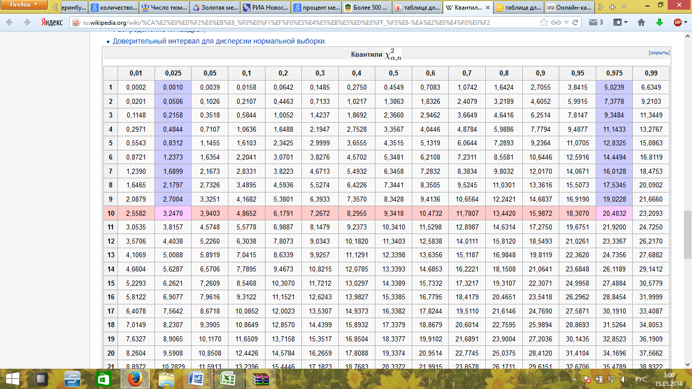
Определим
квантиль распределения
 ,
,
для этого воспользуемся специальной
таблицей:
 ,
,
![]()

 12,8325
 0,8312
-
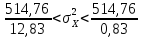
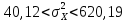
Подставим
найденные значения в формулу из пункта
1):
Для
Х:
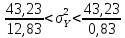
Для
У:

Доверительный интервал для корреляции
Найдем
доверительный интервал для корреляции
при условии, что выборка получена из
генеральной совокупности, r
– выборочный коэффициент корреляции.
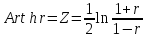
Для
расчета доверительного интервала
применим формулу:
-
Рассчитаем
:
 :
:
-
возьмем
из таблицы квантилей нормального
распределения:
 возьмем

-
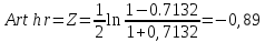
Подставим
все в формулы:
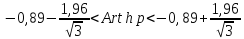
-
Найдем
с помощью таблицы гиперболических
тангенсов:
 с помощью таблицы гиперболических
-
Проверка гипотез
Таким
образом было установлено, что между
заработной платой преподавателей
средних школ и количеством
выпускников-медалистов существует
связь. Искомая
корреляция равна -0.7132. Это
высокая степень взаимосвязи – значения
коэффициента корреляции находится в
пределах от 0,7 до 0,99. Нам удалось выявить
зависимость, но результаты оказались
крайне неожиданными. Чем выше средняя
заработная плата по субъекту РФ, тем
меньше медалистов в этом субъекте.
Почему получились такие результаты,
нам остается только гадать. Да и не было
нашей целью объяснять почему именно
так. Мы должны были, ради личного интереса,
посмотреть есть ли связь.
-
Регрессия
Любая
нелинейная регрессия, в которой уравнение
регрессии для изменений в одной переменной
(у) как функции t изменений в другой (х)
является квадратичным, кубическим или
уравнение более высокого порядка. Хотя
математически всегда возможно получить
уравнение регрессии, которое будет
соответствовать каждой «загогулине»
кривой, большинство этих пертурбаций
возникает в результате ошибок в
составлении выборки или измерении, и
такое «совершенное» соответствие
ничего не дает. Не всегда легко определить,
соответствует ли криволинейная регрессия
набору данных, хотя существуют
статистические тесты для определения
того, значительно ли увеличивает каждая
более высокая степень уравнения степ
совпадения этого набора данных.
Теперь,
будем считать, что выборочная криволинейная
регрессия определяется уравнением:

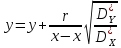
Коэффициенты
называются выборочными коэффициентами
регрессии.
Из
ранее изученных пунктов, нам известны
следующие параметры:
х
= 20,35
у
= 9,47
 =
=
85,79
 =
=
7,21
 =
=
-0.71
Теперь
мы можем подставить все значения в
уравнение:
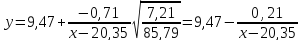
В
итоге имеем:
Вывод
Итак,
в ходе исследований и расчетов,
проделанных в данной работе, мы увидели,
что есть обратная зависимость между
заработной платой преподавателей
средней школы и количеством выпускников
–медалистов. Я не берусь объяснять
причины данного факта, их крайне много
и они довольно субъективны. Мы выяснили,
что такая зависимость довольно сильная.
Соседние файлы в папке МДЗ
- #
- #
- #
- #
- #
- #
- #
- #
- #
- #
- #
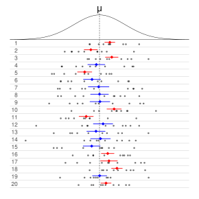
Each row of points is a sample from the same normal distribution. The colored lines are 50% confidence intervals for the mean, μ. At the center of each interval is the sample mean, marked with a diamond. The blue intervals contain the population mean, and the red ones do not.
In frequentist statistics, a confidence interval (CI) is a range of estimates for an unknown parameter. A confidence interval is computed at a designated confidence level; the 95% confidence level is most common, but other levels, such as 90% or 99%, are sometimes used.[1][2] The confidence level represents the long-run proportion of CIs (at the given confidence level) that theoretically contain the true value of the parameter. For example, out of all intervals computed at the 95% level, 95% of them should contain the parameter’s true value.[3]
Factors affecting the width of the CI include the sample size, the variability in the sample, and the confidence level.[4] All else being the same, a larger sample produces a narrower confidence interval, greater variability in the sample produces a wider confidence interval, and a higher confidence level produces a wider confidence interval.[5]
Definition[edit]
Let X be a random sample from a probability distribution with statistical parameter θ, which is a quantity to be estimated, and φ, representing quantities that are not of immediate interest. A confidence interval for the parameter θ, with confidence level or coefficient γ, is an interval  determined by random variables
  and
and  with the property:

The number γ, whose typical value is close to but not greater than 1, is sometimes given in the form  (or as a percentage
  ), where
  is a small positive number, often 0.05 .
It is important for the bounds and to be specified in such a way that as long as X is collected randomly, every time we compute a confidence interval, there is probability γ that it would contain θ, the true value of the parameter being estimated. This should hold true for any actual θ and φ.[2]
Approximate confidence intervals[edit]
In many applications, confidence intervals that have exactly the required confidence level are hard to construct, but approximate intervals can be computed. The rule for constructing the interval may be accepted as providing a confidence interval at level  if
if

to an acceptable level of approximation. Alternatively, some authors[6] simply require that

which is useful if the probabilities are only partially identified or imprecise, and also when dealing with discrete distributions. Confidence limits of form
- and


are called conservative;[7](p 210) accordingly, one speaks of conservative confidence intervals and, in general, regions.
Desired properties[edit]
When applying standard statistical procedures, there will often be standard ways of constructing confidence intervals. These will have been devised so as to meet certain desirable properties, which will hold given that the assumptions on which the procedure relies are true. These desirable properties may be described as: validity, optimality, and invariance.
Of the three, «validity» is most important, followed closely by «optimality». «Invariance» may be considered as a property of the method of derivation of a confidence interval, rather than of the rule for constructing the interval. In non-standard applications, these same desirable properties would be sought:
Validity[edit]
This means that the nominal coverage probability (confidence level) of the confidence interval should hold, either exactly or to a good approximation.
Optimality[edit]
This means that the rule for constructing the confidence interval should make as much use of the information in the data-set as possible.
Recall that one could throw away half of a dataset and still be able to derive a valid confidence interval. One way of assessing optimality is by the length of the interval so that a rule for constructing a confidence interval is judged better than another if it leads to intervals whose lengths are typically shorter.
Invariance[edit]
In many applications, the quantity being estimated might not be tightly defined as such.
For example, a survey might result in an estimate of the median income in a population, but it might equally be considered as providing an estimate of the logarithm of the median income, given that this is a common scale for presenting graphical results. It would be desirable that the method used for constructing a confidence interval for the median income would give equivalent results when applied to constructing a confidence interval for the logarithm of the median income: Specifically the values at the ends of the latter interval would be the logarithms of the values at the ends of former interval.
Methods of derivation[edit]
For non-standard applications, there are several routes that might be taken to derive a rule for the construction of confidence intervals. Established rules for standard procedures might be justified or explained via several of these routes. Typically a rule for constructing confidence intervals is closely tied to a particular way of finding a point estimate of the quantity being considered.
Summary statistics[edit]
This is closely related to the method of moments for estimation. A simple example arises where the quantity to be estimated is the population mean, in which case a natural estimate is the sample mean. Similarly, the sample variance can be used to estimate the population variance. A confidence interval for the true mean can be constructed centered on the sample mean with a width which is a multiple of the square root of the sample variance.
Likelihood theory[edit]
Estimates can be constructed using the maximum likelihood principle, the likelihood theory for this provides two ways of constructing confidence intervals or confidence regions for the estimates.
Estimating equations[edit]
The estimation approach here can be considered as both a generalization of the method of moments and a generalization of the maximum likelihood approach. There are corresponding generalizations of the results of maximum likelihood theory that allow confidence intervals to be constructed based on estimates derived from estimating equations.[citation needed]
Hypothesis testing[edit]
If hypothesis tests are available for general values of a parameter, then confidence intervals/regions can be constructed by including in the 100 p % confidence region all those points for which the hypothesis test of the null hypothesis that the true value is the given value is not rejected at a significance level of (1 − p) .[7](§ 7.2 (iii))
Bootstrapping[edit]
In situations where the distributional assumptions for the above methods are uncertain or violated, resampling methods allow construction of confidence intervals or prediction intervals. The observed data distribution and the internal correlations are used as the surrogate for the correlations in the wider population.
Central limit theorem[edit]
The central limit theorem is a refinement of the law of large numbers. For a large number of independent identically distributed random variables  with finite variance, the average
  approximately has a normal distribution, no matter what the distribution of the
  is, with the approximation roughly improving in proportion to
  [2]
[2]
Example[edit]
Suppose {X1, …, Xn} is an independent sample from a normally distributed population with unknown parameters mean μ and variance σ2. Let


Where X is the sample mean, and S2 is the sample variance. Then

has a Student’s t distribution with n − 1 degrees of freedom.[8] Note that the distribution of T does not depend on the values of the unobservable parameters μ and σ2; i.e., it is a pivotal quantity. Suppose we wanted to calculate a 95% confidence interval for μ. Then, denoting c as the 97.5th percentile of this distribution,

Note that «97.5th» and «0.95» are correct in the preceding expressions. There is a 2.5% chance that  will be less than
  and a 2.5% chance that it will be larger than
  . Thus, the probability that will be between and is 95%.
Consequently,

and we have a theoretical (stochastic) 95% confidence interval for μ.
After observing the sample we find values x for X and s for S, from which we compute the confidence interval
![{displaystyle left[{bar {x}}-{frac {cs}{sqrt {n}}},{bar {x}}+{frac {cs}{sqrt {n}}}right].}](https://wikimedia.org/api/rest_v1/media/math/render/svg/02a90d533cc8ae393c6949495405824f49865b80)

In this bar chart, the top ends of the brown bars indicate observed means and the red line segments («error bars») represent the confidence intervals around them. Although the error bars are shown as symmetric around the means, that is not always the case. In most graphs, the error bars do not represent confidence intervals (e.g., they often represent standard errors or standard deviations)
Interpretation[edit]
Various interpretations of a confidence interval can be given (taking the 95% confidence interval as an example in the following).
- The confidence interval can be expressed in terms of a long-run frequency in repeated samples (or in resampling): «Were this procedure to be repeated on numerous samples, the proportion of calculated 95% confidence intervals that encompassed the true value of the population parameter would tend toward 95%.»[9]
- The confidence interval can be expressed in terms of probability with respect to a single theoretical (yet to be realized) sample: «There is a 95% probability that the 95% confidence interval calculated from a given future sample will cover the true value of the population parameter.» [10] This essentially reframes the «repeated samples» interpretation as a probability rather than a frequency. See Neyman construction.
- The confidence interval can be expressed in terms of statistical significance, e.g.: «The 95% confidence interval represents values that are not statistically significantly different from the point estimate at the .05 level«.[11]

Interpretation of the 95% confidence interval in terms of statistical significance.
Common misunderstandings[edit]
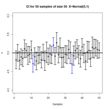
Plot of 50 confidence intervals from 50 samples generated from a normal distribution.
See also: § Counterexamples
Confidence intervals and levels are frequently misunderstood, and published studies have shown that even professional scientists often misinterpret them.[12][13][14][15][16][17]
- A 95% confidence level does not mean that for a given realized interval there is a 95% probability that the population parameter lies within the interval (i.e., a 95% probability that the interval covers the population parameter).[18] According to the strict frequentist interpretation, once an interval is calculated, this interval either covers the parameter value or it does not; it is no longer a matter of probability. The 95% probability relates to the reliability of the estimation procedure, not to a specific calculated interval.[19] Neyman himself (the original proponent of confidence intervals) made this point in his original paper:[10]
It will be noticed that in the above description, the probability statements refer to the problems of estimation with which the statistician will be concerned in the future. In fact, I have repeatedly stated that the frequency of correct results will tend to α. Consider now the case when a sample is already drawn, and the calculations have given [particular limits]. Can we say that in this particular case the probability of the true value [falling between these limits] is equal to α? The answer is obviously in the negative. The parameter is an unknown constant, and no probability statement concerning its value may be made…
- Deborah Mayo expands on this further as follows:[20]
It must be stressed, however, that having seen the value [of the data], Neyman–Pearson theory never permits one to conclude that the specific confidence interval formed covers the true value of 0 with either (1 − α)100% probability or (1 − α)100% degree of confidence. Seidenfeld’s remark seems rooted in a (not uncommon) desire for Neyman–Pearson confidence intervals to provide something which they cannot legitimately provide; namely, a measure of the degree of probability, belief, or support that an unknown parameter value lies in a specific interval. Following Savage (1962), the probability that a parameter lies in a specific interval may be referred to as a measure of final precision. While a measure of final precision may seem desirable, and while confidence levels are often (wrongly) interpreted as providing such a measure, no such interpretation is warranted. Admittedly, such a misinterpretation is encouraged by the word ‘confidence’.
- A 95% confidence level does not mean that 95% of the sample data lie within the confidence interval.
- A confidence interval is not a definitive range of plausible values for the sample parameter, though it is often heuristically taken as a range of plausible values.
- A particular confidence level of 95% calculated from an experiment does not mean that there is a 95% probability of a sample parameter from a repeat of the experiment falling within this interval.[16]
Counterexamples[edit]
Since confidence interval theory was proposed, a number of counter-examples to the theory have been developed to show how the interpretation of confidence intervals can be problematic, at least if one interprets them naïvely.
Confidence procedure for uniform location[edit]
Welch[21] presented an example which clearly shows the difference between the theory of confidence intervals and other theories of interval estimation (including Fisher’s fiducial intervals and objective Bayesian intervals). Robinson[22] called this example «[p]ossibly the best known counterexample for Neyman’s version of confidence interval theory.» To Welch, it showed the superiority of confidence interval theory; to critics of the theory, it shows a deficiency. Here we present a simplified version.
Suppose that  are independent observations from a Uniform(θ − 1/2, θ + 1/2) distribution. Then the optimal 50% confidence procedure for
  is[23]
![{displaystyle {bar {X}}pm {begin{cases}{dfrac {|X_{1}-X_{2}|}{2}}&{text{if }}|X_{1}-X_{2}|<1/2\[8pt]{dfrac {1-|X_{1}-X_{2}|}{2}}&{text{if }}|X_{1}-X_{2}|geq 1/2.end{cases}}}](https://wikimedia.org/api/rest_v1/media/math/render/svg/80260117bd9ee1f05d0928e0b5697663a297ecbc)
A fiducial or objective Bayesian argument can be used to derive the interval estimate

which is also a 50% confidence procedure. Welch showed that the first confidence procedure dominates the second, according to desiderata from confidence interval theory; for every  , the probability that the first procedure contains
  is less than or equal to the probability that the second procedure contains . The average width of the intervals from the first procedure is less than that of the second. Hence, the first procedure is preferred under classical confidence interval theory.
However, when  , intervals from the first procedure are guaranteed to contain the true value : Therefore, the nominal 50% confidence coefficient is unrelated to the uncertainty we should have that a specific interval contains the true value. The second procedure does not have this property.
Moreover, when the first procedure generates a very short interval, this indicates that are very close together and hence only offer the information in a single data point. Yet the first interval will exclude almost all reasonable values of the parameter due to its short width. The second procedure does not have this property.
The two counter-intuitive properties of the first procedure—100% coverage when are far apart and almost 0% coverage when are close together—balance out to yield 50% coverage on average. However, despite the first procedure being optimal, its intervals offer neither an assessment of the precision of the estimate nor an assessment of the uncertainty one should have that the interval contains the true value.
This counter-example is used to argue against naïve interpretations of confidence intervals. If a confidence procedure is asserted to have properties beyond that of the nominal coverage (such as relation to precision, or a relationship with Bayesian inference), those properties must be proved; they do not follow from the fact that a procedure is a confidence procedure.
Confidence procedure for ω2[edit]
Steiger[24] suggested a number of confidence procedures for common effect size measures in ANOVA. Morey et al.[18] point out that several of these confidence procedures, including the one for ω2, have the property that as the F statistic becomes increasingly small—indicating misfit with all possible values of ω2—the confidence interval shrinks and can even contain only the single value ω2 = 0; that is, the CI is infinitesimally narrow (this occurs when  for a
for a  CI).
CI).
This behavior is consistent with the relationship between the confidence procedure and significance testing: as F becomes so small that the group means are much closer together than we would expect by chance, a significance test might indicate rejection for most or all values of ω2. Hence the interval will be very narrow or even empty (or, by a convention suggested by Steiger, containing only 0). However, this does not indicate that the estimate of ω2 is very precise. In a sense, it indicates the opposite: that the trustworthiness of the results themselves may be in doubt. This is contrary to the common interpretation of confidence intervals that they reveal the precision of the estimate.
History[edit]
Confidence intervals were introduced by Jerzy Neyman in 1937.[25] Statisticians quickly took to the idea, but adoption by scientists was more gradual. Some authors in medical journals promoted confidence intervals as early as the 1970s. Despite this, confidence intervals were rarely used until the following decade, when they quickly became standard.[26] By the late 1980s, medical journals began to require the reporting of confidence intervals.[27]
See also[edit]
- CLs upper limits (particle physics)
- 68–95–99.7 rule
- Confidence band, an interval estimate for a curve
- Confidence distribution
- Confidence region, a higher dimensional generalization
- Credence (statistics) – measure of belief strength used in statistics
- Credible interval, a Bayesian alternative for interval estimation
- Cumulative distribution function-based nonparametric confidence interval
- Error bar – Graphical representations of the variability of data
- Estimation statistics – Data analysis approach in frequentist statistics
- Margin of error, the CI halfwidth
- p-value – Function of the observed sample results
- Prediction interval, an interval estimate for a random variable
- Probable error
- Robust confidence intervals
Confidence interval for specific distributions[edit]
- Confidence interval for binomial distribution
- Confidence interval for exponent of the power law distribution
- Confidence interval for mean of the exponential distribution
- Confidence interval for mean of the Poisson distribution
- Confidence intervals for mean and variance of the normal distribution
References[edit]
- ^ Zar, Jerrold H. (199). Biostatistical Analysis (4th ed.). Upper Saddle River, N.J.: Prentice Hall. pp. 43–45. ISBN 978-0130815422. OCLC 39498633.
- ^ a b c Dekking, Frederik Michel; Kraaikamp, Cornelis; Lopuhaä, Hendrik Paul; Meester, Ludolf Erwin (2005). «A Modern Introduction to Probability and Statistics». Springer Texts in Statistics. doi:10.1007/1-84628-168-7. ISBN 978-1-85233-896-1. ISSN 1431-875X.
- ^ Illowsky, Barbara. Introductory statistics. Dean, Susan L., 1945-, Illowsky, Barbara., OpenStax College. Houston, Texas. ISBN 978-1-947172-05-0. OCLC 899241574.
- ^ Hazra, Avijit (October 2017). «Using the confidence interval confidently». Journal of Thoracic Disease. 9 (10): 4125–4130. doi:10.21037/jtd.2017.09.14. ISSN 2072-1439. PMC 5723800. PMID 29268424.
- ^ Khare, Vikas; Nema, Savita; Baredar, Prashant (2020). Ocean Energy Modeling and Simulation with Big Data Computational Intelligence for System Optimization and Grid Integration. ISBN 978-0-12-818905-4. OCLC 1153294021.
- ^ Roussas, George G. (1997). A Course in Mathematical Statistics (2nd ed.). Academic Press. p. 397.
- ^ a b Cox, D.R.; Hinkley, D.V. (1974). Theoretical Statistics. Chapman & Hall.
- ^ Rees. D.G. (2001) Essential Statistics, 4th Edition, Chapman and Hall/CRC. ISBN 1-58488-007-4 (Section 9.5)
- ^ Cox D.R., Hinkley D.V. (1974) Theoretical Statistics, Chapman & Hall, p49, p209
- ^ a b Neyman, J. (1937). «Outline of a Theory of Statistical Estimation Based on the Classical Theory of Probability». Philosophical Transactions of the Royal Society A. 236 (767): 333–380. Bibcode:1937RSPTA.236..333N. doi:10.1098/rsta.1937.0005. JSTOR 91337.
- ^ Cox D.R., Hinkley D.V. (1974) Theoretical Statistics, Chapman & Hall, pp 214, 225, 233
- ^ Kalinowski, Pawel (2010). «Identifying Misconceptions about Confidence Intervals» (PDF). Retrieved 2021-12-22.
- ^ «Archived copy» (PDF). Archived from the original (PDF) on 2016-03-04. Retrieved 2014-09-16.
{{cite web}}: CS1 maint: archived copy as title (link) - ^ Hoekstra, R., R. D. Morey, J. N. Rouder, and E-J. Wagenmakers, 2014. Robust misinterpretation of confidence intervals. Psychonomic Bulletin Review, in press. [1]
- ^ Scientists’ grasp of confidence intervals doesn’t inspire confidence, Science News, July 3, 2014
- ^ a b Greenland, Sander; Senn, Stephen J.; Rothman, Kenneth J.; Carlin, John B.; Poole, Charles; Goodman, Steven N.; Altman, Douglas G. (April 2016). «Statistical tests, P values, confidence intervals, and power: a guide to misinterpretations». European Journal of Epidemiology. 31 (4): 337–350. doi:10.1007/s10654-016-0149-3. ISSN 0393-2990. PMC 4877414. PMID 27209009.
- ^ Helske, Jouni; Helske, Satu; Cooper, Matthew; Ynnerman, Anders; Besancon, Lonni (2021-08-01). «Can Visualization Alleviate Dichotomous Thinking? Effects of Visual Representations on the Cliff Effect». IEEE Transactions on Visualization and Computer Graphics. Institute of Electrical and Electronics Engineers (IEEE). 27 (8): 3397–3409. arXiv:2002.07671. doi:10.1109/tvcg.2021.3073466. ISSN 1077-2626. PMID 33856998. S2CID 233230810.
- ^ a b Morey, R. D.; Hoekstra, R.; Rouder, J. N.; Lee, M. D.; Wagenmakers, E.-J. (2016). «The Fallacy of Placing Confidence in Confidence Intervals». Psychonomic Bulletin & Review. 23 (1): 103–123. doi:10.3758/s13423-015-0947-8. PMC 4742505. PMID 26450628.
- ^ «1.3.5.2. Confidence Limits for the Mean». nist.gov. Archived from the original on 2008-02-05. Retrieved 2014-09-16.
- ^ Mayo, D. G. (1981) «In defence of the Neyman–Pearson theory of confidence intervals», Philosophy of Science, 48 (2), 269–280. JSTOR 187185
- ^ Welch, B. L. (1939). «On Confidence Limits and Sufficiency, with Particular Reference to Parameters of Location». The Annals of Mathematical Statistics. 10 (1): 58–69. doi:10.1214/aoms/1177732246. JSTOR 2235987.
- ^ Robinson, G. K. (1975). «Some Counterexamples to the Theory of Confidence Intervals». Biometrika. 62 (1): 155–161. doi:10.2307/2334498. JSTOR 2334498.
- ^ Pratt, J. W. (1961). «Book Review: Testing Statistical Hypotheses. by E. L. Lehmann». Journal of the American Statistical Association. 56 (293): 163–167. doi:10.1080/01621459.1961.10482103. JSTOR 2282344.
- ^ Steiger, J. H. (2004). «Beyond the F test: Effect size confidence intervals and tests of close fit in the analysis of variance and contrast analysis». Psychological Methods. 9 (2): 164–182. doi:10.1037/1082-989x.9.2.164. PMID 15137887.
- ^ [Neyman, J., 1937. Outline of a theory of statistical estimation based on the classical theory of probability. Philosophical Transactions of the Royal Society of London. Series A, Mathematical and Physical Sciences, 236(767), pp.333-380]
- ^ Altman, Douglas G. (1991). «Statistics in medical journals: Developments in the 1980s». Statistics in Medicine. 10 (12): 1897–1913. doi:10.1002/sim.4780101206. ISSN 1097-0258. PMID 1805317.
- ^ Sandercock, Peter A.G. (2015). «Short History of Confidence Intervals». Stroke. Ovid Technologies (Wolters Kluwer Health). 46 (8): e184-7. doi:10.1161/strokeaha.115.007750. ISSN 0039-2499. PMID 26106115.
Bibliography[edit]
- Fisher, R.A. (1956) Statistical Methods and Scientific Inference. Oliver and Boyd, Edinburgh. (See p. 32.)
- Freund, J.E. (1962) Mathematical Statistics Prentice Hall, Englewood Cliffs, NJ. (See pp. 227–228.)
- Hacking, I. (1965) Logic of Statistical Inference. Cambridge University Press, Cambridge. ISBN 0-521-05165-7
- Keeping, E.S. (1962) Introduction to Statistical Inference. D. Van Nostrand, Princeton, NJ.
- Kiefer, J. (1977). «Conditional Confidence Statements and Confidence Estimators (with discussion)». Journal of the American Statistical Association. 72 (360a): 789–827. doi:10.1080/01621459.1977.10479956. JSTOR 2286460.
- Mayo, D. G. (1981) «In defence of the Neyman–Pearson theory of confidence intervals», Philosophy of Science, 48 (2), 269–280. JSTOR 187185
- Neyman, J. (1937) «Outline of a Theory of Statistical Estimation Based on the Classical Theory of Probability» Philosophical Transactions of the Royal Society of London A, 236, 333–380. (Seminal work.)
- Robinson, G.K. (1975). «Some Counterexamples to the Theory of Confidence Intervals». Biometrika. 62 (1): 155–161. doi:10.1093/biomet/62.1.155. JSTOR 2334498.
- Savage, L. J. (1962), The Foundations of Statistical Inference. Methuen, London.
- Smithson, M. (2003) Confidence intervals. Quantitative Applications in the Social Sciences Series, No. 140. Belmont, CA: SAGE Publications. ISBN 978-0-7619-2499-9.
- Mehta, S. (2014) Statistics Topics ISBN 978-1-4992-7353-3
- «Confidence estimation», Encyclopedia of Mathematics, EMS Press, 2001 [1994]
- Morey, R. D.; Hoekstra, R.; Rouder, J. N.; Lee, M. D.; Wagenmakers, E.-J. (2016). «The fallacy of placing confidence in confidence intervals». Psychonomic Bulletin & Review. 23 (1): 103–123. doi:10.3758/s13423-015-0947-8. PMC 4742505. PMID 26450628.
External links[edit]
- The Exploratory Software for Confidence Intervals tutorial programs that run under Excel
- Confidence interval calculators for R-Squares, Regression Coefficients, and Regression Intercepts
- Weisstein, Eric W. «Confidence Interval». MathWorld.
- CAUSEweb.org Many resources for teaching statistics including Confidence Intervals.
- An interactive introduction to Confidence Intervals
- Confidence Intervals: Confidence Level, Sample Size, and Margin of Error by Eric Schulz, the Wolfram Demonstrations Project.
- Confidence Intervals in Public Health. Straightforward description with examples and what to do about small sample sizes or rates near 0.
Each row of points is a sample from the same normal distribution. The colored lines are 50% confidence intervals for the mean, μ. At the center of each interval is the sample mean, marked with a diamond. The blue intervals contain the population mean, and the red ones do not.
In frequentist statistics, a confidence interval (CI) is a range of estimates for an unknown parameter. A confidence interval is computed at a designated confidence level; the 95% confidence level is most common, but other levels, such as 90% or 99%, are sometimes used.[1][2] The confidence level represents the long-run proportion of CIs (at the given confidence level) that theoretically contain the true value of the parameter. For example, out of all intervals computed at the 95% level, 95% of them should contain the parameter’s true value.[3]
Factors affecting the width of the CI include the sample size, the variability in the sample, and the confidence level.[4] All else being the same, a larger sample produces a narrower confidence interval, greater variability in the sample produces a wider confidence interval, and a higher confidence level produces a wider confidence interval.[5]
Definition[edit]
Let X be a random sample from a probability distribution with statistical parameter θ, which is a quantity to be estimated, and φ, representing quantities that are not of immediate interest. A confidence interval for the parameter θ, with confidence level or coefficient γ, is an interval determined by random variables and with the property:
The number γ, whose typical value is close to but not greater than 1, is sometimes given in the form (or as a percentage ), where is a small positive number, often 0.05 .
It is important for the bounds and to be specified in such a way that as long as X is collected randomly, every time we compute a confidence interval, there is probability γ that it would contain θ, the true value of the parameter being estimated. This should hold true for any actual θ and φ.[2]
Approximate confidence intervals[edit]
In many applications, confidence intervals that have exactly the required confidence level are hard to construct, but approximate intervals can be computed. The rule for constructing the interval may be accepted as providing a confidence interval at level if
to an acceptable level of approximation. Alternatively, some authors[6] simply require that
which is useful if the probabilities are only partially identified or imprecise, and also when dealing with discrete distributions. Confidence limits of form
- and
are called conservative;[7](p 210) accordingly, one speaks of conservative confidence intervals and, in general, regions.
Desired properties[edit]
When applying standard statistical procedures, there will often be standard ways of constructing confidence intervals. These will have been devised so as to meet certain desirable properties, which will hold given that the assumptions on which the procedure relies are true. These desirable properties may be described as: validity, optimality, and invariance.
Of the three, «validity» is most important, followed closely by «optimality». «Invariance» may be considered as a property of the method of derivation of a confidence interval, rather than of the rule for constructing the interval. In non-standard applications, these same desirable properties would be sought:
Validity[edit]
This means that the nominal coverage probability (confidence level) of the confidence interval should hold, either exactly or to a good approximation.
Optimality[edit]
This means that the rule for constructing the confidence interval should make as much use of the information in the data-set as possible.
Recall that one could throw away half of a dataset and still be able to derive a valid confidence interval. One way of assessing optimality is by the length of the interval so that a rule for constructing a confidence interval is judged better than another if it leads to intervals whose lengths are typically shorter.
Invariance[edit]
In many applications, the quantity being estimated might not be tightly defined as such.
For example, a survey might result in an estimate of the median income in a population, but it might equally be considered as providing an estimate of the logarithm of the median income, given that this is a common scale for presenting graphical results. It would be desirable that the method used for constructing a confidence interval for the median income would give equivalent results when applied to constructing a confidence interval for the logarithm of the median income: Specifically the values at the ends of the latter interval would be the logarithms of the values at the ends of former interval.
Methods of derivation[edit]
For non-standard applications, there are several routes that might be taken to derive a rule for the construction of confidence intervals. Established rules for standard procedures might be justified or explained via several of these routes. Typically a rule for constructing confidence intervals is closely tied to a particular way of finding a point estimate of the quantity being considered.
Summary statistics[edit]
This is closely related to the method of moments for estimation. A simple example arises where the quantity to be estimated is the population mean, in which case a natural estimate is the sample mean. Similarly, the sample variance can be used to estimate the population variance. A confidence interval for the true mean can be constructed centered on the sample mean with a width which is a multiple of the square root of the sample variance.
Likelihood theory[edit]
Estimates can be constructed using the maximum likelihood principle, the likelihood theory for this provides two ways of constructing confidence intervals or confidence regions for the estimates.
Estimating equations[edit]
The estimation approach here can be considered as both a generalization of the method of moments and a generalization of the maximum likelihood approach. There are corresponding generalizations of the results of maximum likelihood theory that allow confidence intervals to be constructed based on estimates derived from estimating equations.[citation needed]
Hypothesis testing[edit]
If hypothesis tests are available for general values of a parameter, then confidence intervals/regions can be constructed by including in the 100 p % confidence region all those points for which the hypothesis test of the null hypothesis that the true value is the given value is not rejected at a significance level of (1 − p) .[7](§ 7.2 (iii))
Bootstrapping[edit]
In situations where the distributional assumptions for the above methods are uncertain or violated, resampling methods allow construction of confidence intervals or prediction intervals. The observed data distribution and the internal correlations are used as the surrogate for the correlations in the wider population.
Central limit theorem[edit]
The central limit theorem is a refinement of the law of large numbers. For a large number of independent identically distributed random variables with finite variance, the average approximately has a normal distribution, no matter what the distribution of the is, with the approximation roughly improving in proportion to [2]
Example[edit]
Suppose {X1, …, Xn} is an independent sample from a normally distributed population with unknown parameters mean μ and variance σ2. Let
Where X is the sample mean, and S2 is the sample variance. Then
has a Student’s t distribution with n − 1 degrees of freedom.[8] Note that the distribution of T does not depend on the values of the unobservable parameters μ and σ2; i.e., it is a pivotal quantity. Suppose we wanted to calculate a 95% confidence interval for μ. Then, denoting c as the 97.5th percentile of this distribution,
Note that «97.5th» and «0.95» are correct in the preceding expressions. There is a 2.5% chance that will be less than and a 2.5% chance that it will be larger than . Thus, the probability that will be between and is 95%.
Consequently,
and we have a theoretical (stochastic) 95% confidence interval for μ.
After observing the sample we find values x for X and s for S, from which we compute the confidence interval
In this bar chart, the top ends of the brown bars indicate observed means and the red line segments («error bars») represent the confidence intervals around them. Although the error bars are shown as symmetric around the means, that is not always the case. In most graphs, the error bars do not represent confidence intervals (e.g., they often represent standard errors or standard deviations)
Interpretation[edit]
Various interpretations of a confidence interval can be given (taking the 95% confidence interval as an example in the following).
- The confidence interval can be expressed in terms of a long-run frequency in repeated samples (or in resampling): «Were this procedure to be repeated on numerous samples, the proportion of calculated 95% confidence intervals that encompassed the true value of the population parameter would tend toward 95%.»[9]
- The confidence interval can be expressed in terms of probability with respect to a single theoretical (yet to be realized) sample: «There is a 95% probability that the 95% confidence interval calculated from a given future sample will cover the true value of the population parameter.» [10] This essentially reframes the «repeated samples» interpretation as a probability rather than a frequency. See Neyman construction.
- The confidence interval can be expressed in terms of statistical significance, e.g.: «The 95% confidence interval represents values that are not statistically significantly different from the point estimate at the .05 level«.[11]
Interpretation of the 95% confidence interval in terms of statistical significance.
Common misunderstandings[edit]
Plot of 50 confidence intervals from 50 samples generated from a normal distribution.
See also: § Counterexamples
Confidence intervals and levels are frequently misunderstood, and published studies have shown that even professional scientists often misinterpret them.[12][13][14][15][16][17]
- A 95% confidence level does not mean that for a given realized interval there is a 95% probability that the population parameter lies within the interval (i.e., a 95% probability that the interval covers the population parameter).[18] According to the strict frequentist interpretation, once an interval is calculated, this interval either covers the parameter value or it does not; it is no longer a matter of probability. The 95% probability relates to the reliability of the estimation procedure, not to a specific calculated interval.[19] Neyman himself (the original proponent of confidence intervals) made this point in his original paper:[10]
It will be noticed that in the above description, the probability statements refer to the problems of estimation with which the statistician will be concerned in the future. In fact, I have repeatedly stated that the frequency of correct results will tend to α. Consider now the case when a sample is already drawn, and the calculations have given [particular limits]. Can we say that in this particular case the probability of the true value [falling between these limits] is equal to α? The answer is obviously in the negative. The parameter is an unknown constant, and no probability statement concerning its value may be made…
- Deborah Mayo expands on this further as follows:[20]
It must be stressed, however, that having seen the value [of the data], Neyman–Pearson theory never permits one to conclude that the specific confidence interval formed covers the true value of 0 with either (1 − α)100% probability or (1 − α)100% degree of confidence. Seidenfeld’s remark seems rooted in a (not uncommon) desire for Neyman–Pearson confidence intervals to provide something which they cannot legitimately provide; namely, a measure of the degree of probability, belief, or support that an unknown parameter value lies in a specific interval. Following Savage (1962), the probability that a parameter lies in a specific interval may be referred to as a measure of final precision. While a measure of final precision may seem desirable, and while confidence levels are often (wrongly) interpreted as providing such a measure, no such interpretation is warranted. Admittedly, such a misinterpretation is encouraged by the word ‘confidence’.
- A 95% confidence level does not mean that 95% of the sample data lie within the confidence interval.
- A confidence interval is not a definitive range of plausible values for the sample parameter, though it is often heuristically taken as a range of plausible values.
- A particular confidence level of 95% calculated from an experiment does not mean that there is a 95% probability of a sample parameter from a repeat of the experiment falling within this interval.[16]
Counterexamples[edit]
Since confidence interval theory was proposed, a number of counter-examples to the theory have been developed to show how the interpretation of confidence intervals can be problematic, at least if one interprets them naïvely.
Confidence procedure for uniform location[edit]
Welch[21] presented an example which clearly shows the difference between the theory of confidence intervals and other theories of interval estimation (including Fisher’s fiducial intervals and objective Bayesian intervals). Robinson[22] called this example «[p]ossibly the best known counterexample for Neyman’s version of confidence interval theory.» To Welch, it showed the superiority of confidence interval theory; to critics of the theory, it shows a deficiency. Here we present a simplified version.
Suppose that are independent observations from a Uniform(θ − 1/2, θ + 1/2) distribution. Then the optimal 50% confidence procedure for is[23]
A fiducial or objective Bayesian argument can be used to derive the interval estimate
which is also a 50% confidence procedure. Welch showed that the first confidence procedure dominates the second, according to desiderata from confidence interval theory; for every , the probability that the first procedure contains is less than or equal to the probability that the second procedure contains . The average width of the intervals from the first procedure is less than that of the second. Hence, the first procedure is preferred under classical confidence interval theory.
However, when , intervals from the first procedure are guaranteed to contain the true value : Therefore, the nominal 50% confidence coefficient is unrelated to the uncertainty we should have that a specific interval contains the true value. The second procedure does not have this property.
Moreover, when the first procedure generates a very short interval, this indicates that are very close together and hence only offer the information in a single data point. Yet the first interval will exclude almost all reasonable values of the parameter due to its short width. The second procedure does not have this property.
The two counter-intuitive properties of the first procedure—100% coverage when are far apart and almost 0% coverage when are close together—balance out to yield 50% coverage on average. However, despite the first procedure being optimal, its intervals offer neither an assessment of the precision of the estimate nor an assessment of the uncertainty one should have that the interval contains the true value.
This counter-example is used to argue against naïve interpretations of confidence intervals. If a confidence procedure is asserted to have properties beyond that of the nominal coverage (such as relation to precision, or a relationship with Bayesian inference), those properties must be proved; they do not follow from the fact that a procedure is a confidence procedure.
Confidence procedure for ω2[edit]
Steiger[24] suggested a number of confidence procedures for common effect size measures in ANOVA. Morey et al.[18] point out that several of these confidence procedures, including the one for ω2, have the property that as the F statistic becomes increasingly small—indicating misfit with all possible values of ω2—the confidence interval shrinks and can even contain only the single value ω2 = 0; that is, the CI is infinitesimally narrow (this occurs when for a CI).
This behavior is consistent with the relationship between the confidence procedure and significance testing: as F becomes so small that the group means are much closer together than we would expect by chance, a significance test might indicate rejection for most or all values of ω2. Hence the interval will be very narrow or even empty (or, by a convention suggested by Steiger, containing only 0). However, this does not indicate that the estimate of ω2 is very precise. In a sense, it indicates the opposite: that the trustworthiness of the results themselves may be in doubt. This is contrary to the common interpretation of confidence intervals that they reveal the precision of the estimate.
History[edit]
Confidence intervals were introduced by Jerzy Neyman in 1937.[25] Statisticians quickly took to the idea, but adoption by scientists was more gradual. Some authors in medical journals promoted confidence intervals as early as the 1970s. Despite this, confidence intervals were rarely used until the following decade, when they quickly became standard.[26] By the late 1980s, medical journals began to require the reporting of confidence intervals.[27]
See also[edit]
- CLs upper limits (particle physics)
- 68–95–99.7 rule
- Confidence band, an interval estimate for a curve
- Confidence distribution
- Confidence region, a higher dimensional generalization
- Credence (statistics) – measure of belief strength used in statistics
- Credible interval, a Bayesian alternative for interval estimation
- Cumulative distribution function-based nonparametric confidence interval
- Error bar – Graphical representations of the variability of data
- Estimation statistics – Data analysis approach in frequentist statistics
- Margin of error, the CI halfwidth
- p-value – Function of the observed sample results
- Prediction interval, an interval estimate for a random variable
- Probable error
- Robust confidence intervals
Confidence interval for specific distributions[edit]
- Confidence interval for binomial distribution
- Confidence interval for exponent of the power law distribution
- Confidence interval for mean of the exponential distribution
- Confidence interval for mean of the Poisson distribution
- Confidence intervals for mean and variance of the normal distribution
References[edit]
- ^ Zar, Jerrold H. (199). Biostatistical Analysis (4th ed.). Upper Saddle River, N.J.: Prentice Hall. pp. 43–45. ISBN 978-0130815422. OCLC 39498633.
- ^ a b c Dekking, Frederik Michel; Kraaikamp, Cornelis; Lopuhaä, Hendrik Paul; Meester, Ludolf Erwin (2005). «A Modern Introduction to Probability and Statistics». Springer Texts in Statistics. doi:10.1007/1-84628-168-7. ISBN 978-1-85233-896-1. ISSN 1431-875X.
- ^ Illowsky, Barbara. Introductory statistics. Dean, Susan L., 1945-, Illowsky, Barbara., OpenStax College. Houston, Texas. ISBN 978-1-947172-05-0. OCLC 899241574.
- ^ Hazra, Avijit (October 2017). «Using the confidence interval confidently». Journal of Thoracic Disease. 9 (10): 4125–4130. doi:10.21037/jtd.2017.09.14. ISSN 2072-1439. PMC 5723800. PMID 29268424.
- ^ Khare, Vikas; Nema, Savita; Baredar, Prashant (2020). Ocean Energy Modeling and Simulation with Big Data Computational Intelligence for System Optimization and Grid Integration. ISBN 978-0-12-818905-4. OCLC 1153294021.
- ^ Roussas, George G. (1997). A Course in Mathematical Statistics (2nd ed.). Academic Press. p. 397.
- ^ a b Cox, D.R.; Hinkley, D.V. (1974). Theoretical Statistics. Chapman & Hall.
- ^ Rees. D.G. (2001) Essential Statistics, 4th Edition, Chapman and Hall/CRC. ISBN 1-58488-007-4 (Section 9.5)
- ^ Cox D.R., Hinkley D.V. (1974) Theoretical Statistics, Chapman & Hall, p49, p209
- ^ a b Neyman, J. (1937). «Outline of a Theory of Statistical Estimation Based on the Classical Theory of Probability». Philosophical Transactions of the Royal Society A. 236 (767): 333–380. Bibcode:1937RSPTA.236..333N. doi:10.1098/rsta.1937.0005. JSTOR 91337.
- ^ Cox D.R., Hinkley D.V. (1974) Theoretical Statistics, Chapman & Hall, pp 214, 225, 233
- ^ Kalinowski, Pawel (2010). «Identifying Misconceptions about Confidence Intervals» (PDF). Retrieved 2021-12-22.
- ^ «Archived copy» (PDF). Archived from the original (PDF) on 2016-03-04. Retrieved 2014-09-16.
{{cite web}}: CS1 maint: archived copy as title (link) - ^ Hoekstra, R., R. D. Morey, J. N. Rouder, and E-J. Wagenmakers, 2014. Robust misinterpretation of confidence intervals. Psychonomic Bulletin Review, in press. [1]
- ^ Scientists’ grasp of confidence intervals doesn’t inspire confidence, Science News, July 3, 2014
- ^ a b Greenland, Sander; Senn, Stephen J.; Rothman, Kenneth J.; Carlin, John B.; Poole, Charles; Goodman, Steven N.; Altman, Douglas G. (April 2016). «Statistical tests, P values, confidence intervals, and power: a guide to misinterpretations». European Journal of Epidemiology. 31 (4): 337–350. doi:10.1007/s10654-016-0149-3. ISSN 0393-2990. PMC 4877414. PMID 27209009.
- ^ Helske, Jouni; Helske, Satu; Cooper, Matthew; Ynnerman, Anders; Besancon, Lonni (2021-08-01). «Can Visualization Alleviate Dichotomous Thinking? Effects of Visual Representations on the Cliff Effect». IEEE Transactions on Visualization and Computer Graphics. Institute of Electrical and Electronics Engineers (IEEE). 27 (8): 3397–3409. arXiv:2002.07671. doi:10.1109/tvcg.2021.3073466. ISSN 1077-2626. PMID 33856998. S2CID 233230810.
- ^ a b Morey, R. D.; Hoekstra, R.; Rouder, J. N.; Lee, M. D.; Wagenmakers, E.-J. (2016). «The Fallacy of Placing Confidence in Confidence Intervals». Psychonomic Bulletin & Review. 23 (1): 103–123. doi:10.3758/s13423-015-0947-8. PMC 4742505. PMID 26450628.
- ^ «1.3.5.2. Confidence Limits for the Mean». nist.gov. Archived from the original on 2008-02-05. Retrieved 2014-09-16.
- ^ Mayo, D. G. (1981) «In defence of the Neyman–Pearson theory of confidence intervals», Philosophy of Science, 48 (2), 269–280. JSTOR 187185
- ^ Welch, B. L. (1939). «On Confidence Limits and Sufficiency, with Particular Reference to Parameters of Location». The Annals of Mathematical Statistics. 10 (1): 58–69. doi:10.1214/aoms/1177732246. JSTOR 2235987.
- ^ Robinson, G. K. (1975). «Some Counterexamples to the Theory of Confidence Intervals». Biometrika. 62 (1): 155–161. doi:10.2307/2334498. JSTOR 2334498.
- ^ Pratt, J. W. (1961). «Book Review: Testing Statistical Hypotheses. by E. L. Lehmann». Journal of the American Statistical Association. 56 (293): 163–167. doi:10.1080/01621459.1961.10482103. JSTOR 2282344.
- ^ Steiger, J. H. (2004). «Beyond the F test: Effect size confidence intervals and tests of close fit in the analysis of variance and contrast analysis». Psychological Methods. 9 (2): 164–182. doi:10.1037/1082-989x.9.2.164. PMID 15137887.
- ^ [Neyman, J., 1937. Outline of a theory of statistical estimation based on the classical theory of probability. Philosophical Transactions of the Royal Society of London. Series A, Mathematical and Physical Sciences, 236(767), pp.333-380]
- ^ Altman, Douglas G. (1991). «Statistics in medical journals: Developments in the 1980s». Statistics in Medicine. 10 (12): 1897–1913. doi:10.1002/sim.4780101206. ISSN 1097-0258. PMID 1805317.
- ^ Sandercock, Peter A.G. (2015). «Short History of Confidence Intervals». Stroke. Ovid Technologies (Wolters Kluwer Health). 46 (8): e184-7. doi:10.1161/strokeaha.115.007750. ISSN 0039-2499. PMID 26106115.
Bibliography[edit]
- Fisher, R.A. (1956) Statistical Methods and Scientific Inference. Oliver and Boyd, Edinburgh. (See p. 32.)
- Freund, J.E. (1962) Mathematical Statistics Prentice Hall, Englewood Cliffs, NJ. (See pp. 227–228.)
- Hacking, I. (1965) Logic of Statistical Inference. Cambridge University Press, Cambridge. ISBN 0-521-05165-7
- Keeping, E.S. (1962) Introduction to Statistical Inference. D. Van Nostrand, Princeton, NJ.
- Kiefer, J. (1977). «Conditional Confidence Statements and Confidence Estimators (with discussion)». Journal of the American Statistical Association. 72 (360a): 789–827. doi:10.1080/01621459.1977.10479956. JSTOR 2286460.
- Mayo, D. G. (1981) «In defence of the Neyman–Pearson theory of confidence intervals», Philosophy of Science, 48 (2), 269–280. JSTOR 187185
- Neyman, J. (1937) «Outline of a Theory of Statistical Estimation Based on the Classical Theory of Probability» Philosophical Transactions of the Royal Society of London A, 236, 333–380. (Seminal work.)
- Robinson, G.K. (1975). «Some Counterexamples to the Theory of Confidence Intervals». Biometrika. 62 (1): 155–161. doi:10.1093/biomet/62.1.155. JSTOR 2334498.
- Savage, L. J. (1962), The Foundations of Statistical Inference. Methuen, London.
- Smithson, M. (2003) Confidence intervals. Quantitative Applications in the Social Sciences Series, No. 140. Belmont, CA: SAGE Publications. ISBN 978-0-7619-2499-9.
- Mehta, S. (2014) Statistics Topics ISBN 978-1-4992-7353-3
- «Confidence estimation», Encyclopedia of Mathematics, EMS Press, 2001 [1994]
- Morey, R. D.; Hoekstra, R.; Rouder, J. N.; Lee, M. D.; Wagenmakers, E.-J. (2016). «The fallacy of placing confidence in confidence intervals». Psychonomic Bulletin & Review. 23 (1): 103–123. doi:10.3758/s13423-015-0947-8. PMC 4742505. PMID 26450628.
External links[edit]
- The Exploratory Software for Confidence Intervals tutorial programs that run under Excel
- Confidence interval calculators for R-Squares, Regression Coefficients, and Regression Intercepts
- Weisstein, Eric W. «Confidence Interval». MathWorld.
- CAUSEweb.org Many resources for teaching statistics including Confidence Intervals.
- An interactive introduction to Confidence Intervals
- Confidence Intervals: Confidence Level, Sample Size, and Margin of Error by Eric Schulz, the Wolfram Demonstrations Project.
- Confidence Intervals in Public Health. Straightforward description with examples and what to do about small sample sizes or rates near 0.
Доверительный интервал для математического ожидания нормальной случайной
величины при неизвестной дисперсии
Пусть
, причем
и
неизвестны. Необходимо построить доверительный интервал,
накрывающий с надежностью
истинное значение параметра
.
Для этого из генеральной
совокупности СВ
извлекается
выборка объема
:
.
1) В качестве точечной
оценки математического ожидания
используется
выборочное среднее
, а в
качестве оценки дисперсии
–
исправленная выборочная дисперсия
которой соответствует стандартное отклонение
.
2) Для нахождения
доверительного интервала строится статистика
имеющая в этом случае распределение Стьюдента с
числом степеней свободы
независимо
от значений параметров
и
.
3) Задается требуемый
уровень значимости
.
4) Применяется следующая
формула расчета вероятности:
где
–
критическая точка распределения Стьюдента, которая находится по таблице критических точек распределения Стьюдента (односторонняя критическая область).
Тогда:
Это означает, что
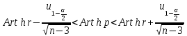
интервал:
накрывает неизвестный
параметр
с
надежностью
Доверительный интервал для математического ожидания
нормальной случайной величины при известной дисперсии
Пусть количественный
признак
генеральной
совокупности имеет нормальное распределение
с
заданной дисперсией
и
неизвестным математическим ожиданием
. Построим
доверительный интервал для
.
1) Пусть для оценки
извлечена
выборка
объема
. Тогда
2) Составим случайную
величину:
Нетрудно показать, что случайная величина
имеет стандартизированное нормальное распределение, то есть:
3) Зададим уровень
значимости
.
4) Применяя формулу нахождения
вероятности отклонения нормальной величины от математического ожидания, имеем:
Это означает, что
доверительный интервал
накрывает неизвестный
параметр
с надежностью
. Точность оценки определяется величиной:
Число
определяется
по таблице значений функции Лапласа из равенства
Окончательно получаем:
Доверительный интервал для
дисперсии нормальной случайной величины при неизвестном математическом ожидании
Пусть
, причем
и
–
неизвестны. Пусть для оценки
извлечена выборка объема
:
.
1) В качестве точечной оценки дисперсии
используется
исправленная выборочная дисперсия
:
которой соответствует стандартное отклонение
.
2) При нахождении
доверительного интервала для дисперсии в этом случае вводится статистика
имеющая
–
распределение с числом степеней свободы
независимо
от значения параметра
.
3) Задается требуемый
уровень значимости
.
4) Тогда, используя таблицу критических точек хи-квадрат распределения, нетрудно указать критические
точки
, для которых будет выполняться следующее
равенство:
Подставив вместо
соответствующее значение, получим:
Получаем доверительный
интервал для неизвестной дисперсии:
Доверительный интервал для
дисперсии нормальной случайной величины при известном математическом ожидании
Пусть
, причем
–
известна, а
–
неизвестна. Пусть для оценки
извлечена выборка объема
:
.
1) В качестве точечной оценки дисперсии
используется выборочная дисперсия:
2) При нахождении
доверительного интервала для дисперсии в этом случае вводится статистика
имеющая
–
распределение с числом степеней свободы
независимо
от значения параметра
.
3) Задается требуемый
уровень значимости
.
4) Тогда, используя таблицу критических точек хи-квадрат распределения,
нетрудно указать критические точки
, для которых будет выполняться следующее
равенство:
Подставив вместо
соответствующее значение, получим:
Получаем доверительный
интервал для неизвестной дисперсии:
Доверительный интервал для
среднего квадратического отклонения
Извлекая квадратный корень:
Положив:
Получим следующий
доверительный интервал для среднего квадратического
отклонения:
Для отыскания
по заданным
и
пользуются специальными таблицами.
Для проверки на нормальность заданного распределения случайной величины можно использовать
правило трех сигм.
Если не находите примера, аналогичного вашему, если сами не успеваете выполнить работу, если впереди экзамен по предмету и нужна помощь — свяжитесь со мной:
ВКонтакте
WhatsApp
Telegram
Я буду работать с вами, над вашей проблемой, пока она не решится.
25 лет я занимаюсь решением задач и потратил на это кучу времени. Вы можете освободить свое, стоит только обратиться за помощью.
Когда нам нужно получить одно число в качестве оценки параметра совокупности, мы используем точечную оценку. Тем не менее, из-за ошибки выборки, точечная оценка не будет в точности равняться параметру совокупности при любом размере данной выборки.
Часто, вместо точечной оценки, более полезным подходом будет найти диапазон значений, в рамках которого, как мы ожидаем, может находится значение искомого параметра с заданным уровнем вероятности.
Этот подход называется интервальной оценкой параметра (англ. ‘interval estimate of parameter’), а доверительный интервал выполняет роль этого диапазона значений.
Определение доверительного интервала.
Доверительный интервал (англ. ‘confidence interval’) представляет собой диапазон, для которого можно утверждать, с заданной вероятностью (1 — alpha ), называемой степенью доверия (или степенью уверенности, англ. ‘degree of confidence’), что он будет содержать оцениваемый параметр.
Этот интервал часто упоминается как (100 (1 — alpha)% ) доверительный интервал для параметра.
Конечные значения доверительного интервала называются нижним и верхним доверительными пределами (или доверительными границами или предельной погрешностью, англ. ‘lower/upper confidence limits’).
В этом чтении, мы имеем дело только с двусторонними доверительными интервалами — доверительные интервалами, для которых мы вычисляем и нижние и верхние пределы.
Кроме того, можно определить два типа односторонних доверительных интервалов для параметра совокупности.
Нижний односторонний доверительный интервал устанавливает только нижний предел. Это означает допущение, что с определенной степенью доверия параметр совокупности равен или превышает нижний предел.
Верхний односторонний доверительный интервал устанавливает только верхний предел. Это означает допущение, что с определенной степенью доверия параметр совокупности меньше или равен верхнему пределу.
Инвестиционные аналитики редко используют односторонние доверительные интервалы.
Доверительные интервалы часто дают либо вероятностную интерпретацию, либо практическую интерпретацию.
При вероятностной интерпретации, мы интерпретируем 95%-ный доверительный интервал для среднего значения совокупности следующим образом.
При повторяющейся выборке, 95% таких доверительных интервалов будут, в конечном счете, включать в себя среднее значение совокупности.
Например, предположим, что мы делаем выборку из совокупности 1000 раз, и на основании каждой выборки мы построим 95%-ный доверительный интервал, используя вычисленное выборочное среднее.
Из-за случайного характера выборок, эти доверительные интервалы отличаются друг от друга, но мы ожидаем, что 95% (или 950) этих интервалов включают неизвестное значение среднего по совокупности.
На практике мы обычно не делаем такие повторяющиеся выборки. Поэтому в практической интерпретации, мы утверждаем, что мы 95% уверены в том, что один 95%-ный доверительный интервал содержит среднее по совокупности.
Мы вправе сделать это заявление, потому что мы знаем, что 95% всех возможных доверительных интервалов, построенных аналогичным образом, будут содержать среднее по совокупности.
Доверительные интервалы, которые мы обсудим в этом чтении, имеют структуры, подобные описанной ниже базовой структуре.
Построение доверительных интервалов.
Доверительный интервал (100 (1 — alpha)% ) для параметра имеет следующую структуру.
Точечная оценка (pm) Фактор надежности (times) Стандартная ошибка
где
- Точечная оценка = точечная оценка параметра (значение выборочной статистики).
- Фактор надежности (англ. ‘reliability factor’) = коэффициент, основанный на предполагаемом распределении точечной оценки и степени доверия ((1 — alpha)) для доверительного интервала.
- Стандартная ошибка = стандартная ошибка выборочной статистики, значение которой получено с помощью точечной оценки.
Величину (Фактор надежности) (times) (Cтандартная ошибка) иногда называют точностью оценки (англ. ‘precision of estimator’). Большие значения этой величины подразумевают более низкую точность оценки параметра совокупности.
Самый базовый доверительный интервал для среднего значения по совокупности появляется тогда, когда мы делаем выборку из нормального распределения с известной дисперсией. Фактор надежности в данном случае на основан стандартном нормальном распределении, которое имеет среднее значение, равное 0 и дисперсию 1.
Стандартная нормальная случайная величина обычно обозначается как (Z). Обозначение (z_alpha ) обозначает такую точку стандартного нормального распределения, в которой (alpha) вероятности остается в правом хвосте.
Например, 0.05 или 5% возможных значений стандартной нормальной случайной величины больше, чем ( z_{0.05} = 1.65 ).
Предположим, что мы хотим построить 95%-ный доверительный интервал для среднего по совокупности, и для этой цели, мы сделали выборку размером 100 из нормально распределенной совокупности с известной дисперсией (sigma^2) = 400 (значит, (sigma) = 20).
Мы рассчитываем выборочное среднее как ( overline X = 25 ). Наша точечная оценка среднего по совокупности, таким образом, 25.
Если мы перемещаем 1.96 стандартных отклонений выше среднего значения нормального распределения, то 0.025 или 2.5% вероятности остается в правом хвосте. В силу симметрии нормального распределения, если мы перемещаем 1.96 стандартных отклонений ниже среднего, то 0.025 или 2.5% вероятности остается в левом хвосте.
В общей сложности, 0.05 или 5% вероятности лежит в двух хвостах и 0.95 или 95% вероятности лежит между ними.
Таким образом, ( z_{0.025} = 1.96) является фактором надежности для этого 95%-ного доверительного интервала. Обратите внимание на связь (100 (1 — alpha)% ) для доверительного интервала и (z_{alpha/2}) для фактора надежности.
Стандартная ошибка среднего значения выборки, заданная Формулой 1, равна:
( sigma_{overline X} = 20 Big / sqrt{100} = 2 )
Доверительный интервал, таким образом, имеет нижний предел:
( overline X — 1.96 sigma_{overline X} ) = 25 — 1.96(2) = 25 — 3.92 = 21.08.
Верхний предел доверительного интервала равен:
( overline X + 1.96sigma_{overline X} ) = 25 + 1.96(2) = 25 + 3.92 = 28.92
95%-ный доверительный интервал для среднего по совокупности охватывает значения от 21.08 до 28.92.
Доверительные интервалы для среднего по совокупности (нормально распределенная совокупность с известной дисперсией).
Доверительный интервал (100 (1 — alpha)% ) для среднего по совокупности ( mu ), когда мы делаем выборку из нормального распределения с известной дисперсией ( sigma^2 ) задается формулой:
( Large dst overline X pm z_{alpha /2}{sigma over sqrt n} ) (Формула 4)
Факторы надежности для наиболее часто используемых доверительных интервалов приведены ниже.
Факторы надежности для доверительных интервалов на основе стандартного нормального распределения.
Мы используем следующие факторы надежности при построении доверительных интервалов на основе стандартного нормального распределения:
- 90%-ные доверительные интервалы: используется (z_{0.05}) = 1.65
- 95%-ные доверительные интервалы: используется (z_{0.025}) = 1.96
- 99%-ные доверительные интервалы: используется (z_{0.005}) = 2.58
На практике, большинство финансовых аналитиков используют значения для (z_{0.05}) и (z_{0.005}), округленные до двух знаков после запятой.
Для справки, более точными значениями для (z_{0.05}) и (z_{0.005}) являются 1.645 и 2.575, соответственно.
Для быстрого расчета 95%-ного доверительного интервала (z_{0.025}) иногда округляют 1.96 до 2.
Эти факторы надежности подчеркивают важный факт о всех доверительных интервалах. По мере того, как мы повышаем степень доверия, доверительный интервал становится все шире и дает нам менее точную информацию о величине, которую мы хотим оценить.
«Чем уверенней мы хотим быть, тем меньше мы должны быть уверены»
см. Freund и Williams (1977), стр. 266.
На практике, допущение о том, что выборочное распределение выборочного среднего, по меньшей мере, приблизительно нормальное, часто является обоснованным, либо потому, что исходное распределение приблизительно нормальное, либо потому что мы имеем большую выборку и поэтому к ней применима центральная предельная теорема.
Однако, на практике, мы редко знаем дисперсию совокупности. Когда дисперсия генеральной совокупности неизвестна, но выборочное среднее, по меньшей мере, приблизительно нормально распределено, у нас есть два приемлемых пути чтобы вычислить доверительные интервалы для среднего значения совокупности.
Вскоре мы обсудим более консервативный подход, который основан на t-распределении Стьюдента (t-распределение, для краткости).
Распределение статистики (t) называется t-распределением Стьюдента (англ. «Student’s t-distribution») из-за псевдонима «Студент» (Student), использованного британским математиком Уильямом Сили Госсеттом, который опубликовал свою работу в 1908 году.
В финансовой литературе, это наиболее часто используемый подход для статистической оценки и проверки статистических гипотез, касающихся среднего значения, когда дисперсия генеральной совокупности не известна, как для малого, так и для большого размер выборки.
Второй подход к доверительным интервалам для среднего по совокупности, основанного на стандартном нормальном распределении, — это z-альтернатива (англ. ‘z-alternative’). Он может быть использован только тогда, когда размер выборки является большим (в общем случае, размер выборки 30 или больше, можно считать большим).
В отличии от доверительного интервала, приведенного в Формуле 4, этот доверительный интервал использует стандартное отклонение выборки (s) при вычислении стандартной ошибки выборочного среднего (по Формуле 2).
Доверительные интервалы для среднего по совокупности — z-альтернатива (большая выборка, дисперсия совокупности неизвестна).
Доверительный интервал (100 (1 — alpha)% ) для среднего по совокупности ( mu ) при выборке из любого распределения с неизвестной дисперсией, когда размер выборки большой, задается формулой:
( Large dst overline X pm z_{alpha /2}{s over sqrt n} ) (Формула 5)
Поскольку этот тип доверительного интервала применяется довольно часто, мы проиллюстрируем его вычисление в Примере 4.
Пример (4) расчета доверительного интервала для среднего по совокупности коэффициентов Шарпа с использованием z-статистики.
Предположим, что инвестиционный аналитик делает случайную выборку акций взаимных фондов США и рассчитывает средний коэффициент Шарпа.
[см. также: CFA — Коэффициент Шарпа]
Размер выборки равен 100, а средний коэффициент Шарпа составляет 0.45. Выборка имеет стандартное отклонение 0.30.
Рассчитайте и интерпретируйте 90-процентный доверительный интервал для среднего по совокупности всех акций взаимных фондов США с использованием фактора надежности на основе стандартного нормального распределения.
Фактор надежности для 90-процентного доверительного интервала, как указано ранее, составляет ( z_{0.05} = 1.65 ).
Доверительный интервал будет равен:
( begin{aligned} & overline X pm z_{0.05}{s over sqrt n } \ &= 0.45 pm 1.65{0.30 over sqrt {100}} \ &= 0.45 pm 1.65(0.03) = 0.45 pm 0.0495 end{aligned} )
Доверительный интервал охватывает значения 0.4005 до 0.4995, или от 0.40 до 0.50, с округлением до двух знаков после запятой. Аналитик может сказать с 90-процентной уверенностью, что интервал включает среднее по совокупности.
В этом примере аналитик не делает никаких конкретных предположений о распределении вероятностей, характеризующем совокупность. Скорее всего, аналитик опирается на центральную предельную теорему для получения приближенного нормального распределения для выборочного среднего.
Как показывает Пример 4, даже если мы не уверены в характере распределения совокупности, мы все еще можем построить доверительные интервалы для среднего по совокупности, если размер выборки достаточно большой, поскольку можем применить центральную предельную теорему.
Концепция степеней свободы.
Обратимся теперь к консервативной альтернативе и используем t-распределение Стьюдента, чтобы построить доверительные интервалы для среднего по совокупности, когда дисперсия генеральной совокупности не известна.
Для доверительных интервалов на основе выборок из нормально распределенных совокупностей с неизвестной дисперсией, теоретически правильный фактор надежности основан на t-распределении. Использование фактора надежности, основанного на t-распределении, имеет важное значение для выборок небольшого размера.
Применение фактора надежности (t) уместно, когда дисперсия генеральной совокупности неизвестна, даже если у нас есть большая выборка и мы можем использовать центральную предельную теорему для обоснования использования фактора надежности (z). В этом случае большой выборки, t-распределение обеспечивает более консервативные (широкие) доверительные интервалы.
t-распределение является симметричным распределением вероятностей и определяется одним параметром, известным как степени свободы (DF, от англ. ‘degrees of freedom’). Каждое значение для числа степеней свободы определяет одно распределение в этом семействе распределений.
Далее мы сравним t-распределения со стандартным нормальным распределением, но сначала мы должны понять концепцию степеней свободы. Мы можем сделать это путем изучения расчета выборочной дисперсии.
Формула 3 дает несмещенную оценку выборочной дисперсии, которую мы используем. Выражение в знаменателе, ( n — 1 ), означающее размер выборки минус 1, это число степеней свободы при расчете дисперсии совокупности с использованием Формулы 3.
Мы также используем ( n — 1 ) как число степеней свободы для определения факторов надежности на основе распределения Стьюдента. Термин «степени свободы» используются, так как мы предполагаем, что в случайной выборке наблюдения отобраны независимо друг от друга. Числитель выборочной дисперсии, однако, использует выборочное среднее.
Каким образом использование выборочного среднего влияет на количество наблюдений, отобранных независимо, для формулы выборочной дисперсии?
При выборке размера 10 и среднем значении в 10%, к примеру, мы можем свободно отобрать только 9 наблюдений. Независимо от отобранных 9 наблюдений, мы всегда можем найти значение для 10-го наблюдения, которое дает среднее значение, равное 10%. С точки зрения формулы выборочной дисперсии, здесь есть 9 степеней свободы.
Учитывая, что мы должны сначала вычислить выборочное среднее от общего числа (n) независимых наблюдений, только (n — 1) наблюдений могут быть отобраны независимо друг от друга для расчета выборочной дисперсии.
Концепция степеней свободы часто применяется в финансовой статистике, и вы встретите ее в последующих чтениях.
t-распределение Стьюдента.
Предположим, что мы делаем выборку из нормального распределения.
Коэффициент (z = (overline X — mu) Big / (sigma big / sqrt n) ) нормально распределен со средним значением 0 и стандартным отклонением 1, однако, коэффициент (t = (overline X — mu) Big / (s big / sqrt n) ) следует t-распределению со средним 0 и (n — 1) степеней свободы.
Коэффициент (t) не является нормальным, поскольку представляет собой отношение двух случайных величин, выборочного среднего и стандартного отклонения выборки.
Определение стандартной нормальной случайной величины включает в себя только одну случайную величину, выборочное среднее. По мере увеличения степеней свободы, однако, t-распределение приближается к стандартному нормальному распределению.
На Рисунке 1 показано стандартное нормальное распределение и два t-распределения, одно с DF = 2 и одно с DF = 8.
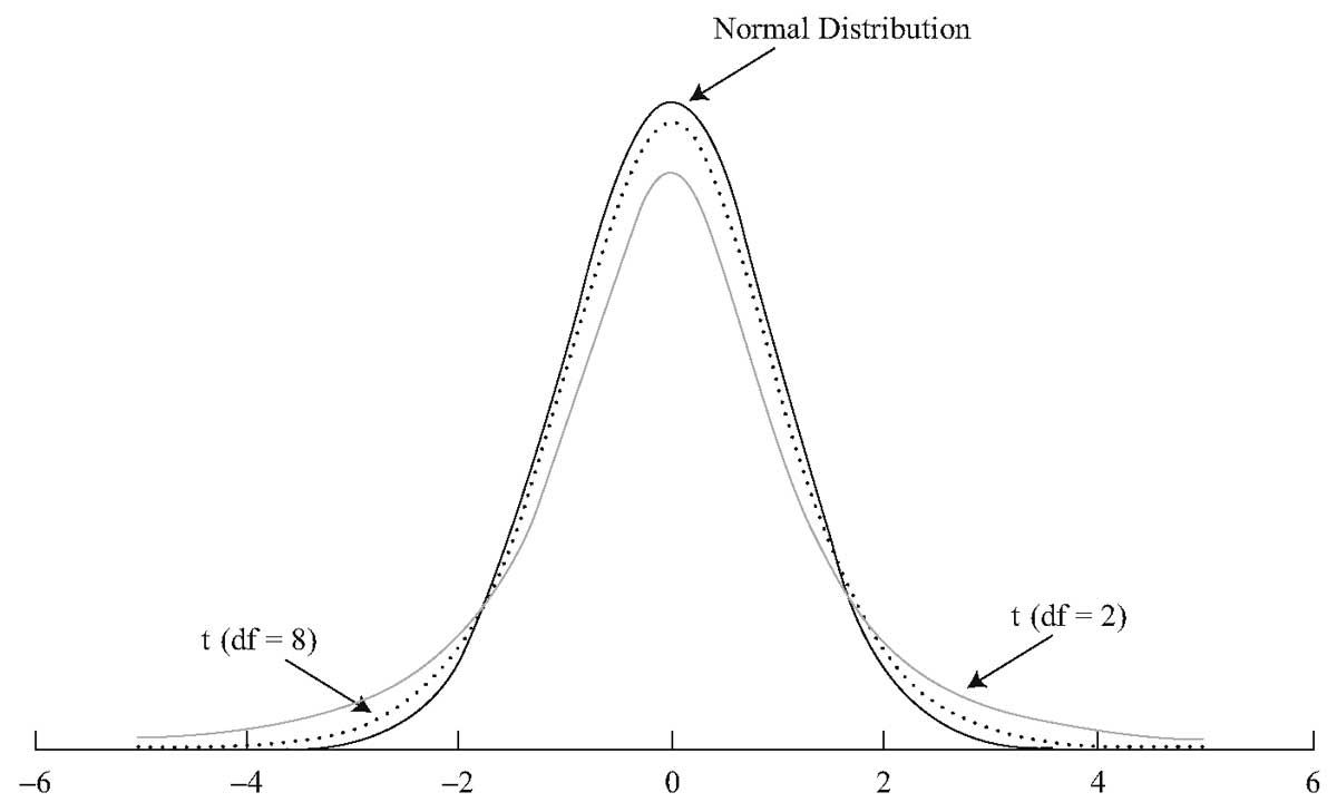 Рисунок (1) t-распределение Стьюдента по сравнению со стандартным нормальным распределением.
Из трех распределений, показанных на Рисунке 1, стандартное нормальное распределение имеет хвосты, которые стремятся к нулю быстрее, чем хвосты двух t-распределений. t-распределение симметрично распределено вокруг среднего нулевого значения, так же как и нормальное распределение.
По мере увеличения степеней свободы, t-распределение приближается к стандартному нормальному распределению. t-распределение с DF = 8 ближе к стандартному нормальному, чем t-распределение с DF = 2.
Помимо области плюс и минус четырех стандартных отклонений от среднего значения, остальная область под стандартным нормальным распределением, как представляется, близка к 0. Однако, оба t-распределения содержать некоторую площадь под каждой кривой за пределом четырех стандартных отклонений.
t-распределения имеют более толстые хвосты, но хвосты t-распределения Стьюдента с DF = 8 сильнее напоминают хвосты нормального распределения. По мере увеличения степеней свободы, хвосты распределения Стьюдента становятся менее толстыми.
Для часто используемых значений распределения Стьюдента составлены таблицы. Например, для каждой степени свободы (t_{0.10}), (t_{0.05}), (t_{0.025}), (t_{0.01}) и (t_{0.005}) значения будут такими, что соответственно, 0.10, 0.05, 0.025, 0.01 и 0.005 вероятности останется в правом хвосте для заданного числа степеней свободы.
Значения (t_{0.10}), (t_{0.05}), (t_{0.025}), (t_{0.01}) и (t_{0.005}) также называют односторонними критическими значениями t на значимых уровнях 0.10, 0.05, 0.025, 0.01 и 0.005, для указанного числа степеней свободы.
Например,
для DF = 30,
(t_{0.10}) = 1.310,
(t_{0.05}) = 1.697,
(t_{0.025}) = 2.042,
(t_{0.01}) = 2.457,
(t_{0.005}) = 2.750.
Приведем форму доверительных интервалов для среднего по совокупности, используя распределение Стьюдента.
Доверительные интервалы для среднего по совокупности (дисперсия совокупности неизвестна) — t-распределение.
Если мы делаем выборку из генеральной совокупности с неизвестной дисперсией и соблюдается одно из перечисленных ниже условий:
- выборка является большой, или
- выборка небольшая, но совокупность имеет нормальное распределение, или приблизительно нормально распределена,
то доверительный интервал (100 (1 — alpha)% ) для среднего совокупности ( mu ) задается формулой:
( Large dst overline X pm t_{alpha /2}{s over sqrt n} ) (Формула 6)
где число степеней свободы для ( t_{alpha /2}) равно ( n-1 ), а ( n ) — это размер выборки.
Пример 5 использует данные Примера 4, но применяет t-статистику, а не z-статистику, чтобы рассчитать доверительный интервал для среднего значения совокупности коэффициентов Шарпа.
Пример (5) расчета доверительного интервала для среднего по совокупности коэффициентов Шарпа с использованием t-статистики.
Как и в Примере 4, инвестиционный аналитик стремится вычислить 90-процентный доверительный интервал для среднего по совокупности коэффициентов Шарпа, основанных на случайной выборке из 100 взаимных фондов США.
Выборочное среднее коэффициентов Шарпа составляет 0.45, а выборочное стандартное отклонение — 0.30.
Теперь, признав, что дисперсия генеральной совокупности распределения коэффициентов Шарпа неизвестна, аналитик решает вычислить доверительный интервал, используя теоретически правильную t-статистику.
Поскольку размер выборки равен 100, DF = 99. Используя таблицу степеней свободы, мы находим, что (t_{0.05}) = 1.66.
Этот фактор надежности немного больше, чем фактор надежности (z_{0.05}) = 1.65, который был использован в Примере 4.
Доверительный интервал будет:
( begin{aligned} & overline X pm t_{0.05}{s over sqrt n } \ &= 0.45 pm 1.66{0.30 over sqrt {100}} \ &= 0.45 pm 1.66(0.03) = 0.45 pm 0.0498 end{aligned} )
Доверительный интервал охватывает значения 0.4002 до 0.4998, или 0.40 до 0.50, с двумя знаками после запятой. При округлении до двух знаков после запятой, доверительный интервал не изменился по сравнению с Примером 4.
В Таблице 3 приведены различные факторы надежности, которые мы использовали.
|
Выборка из: |
Статистика для выборки малого размера |
Статистика для выборки большого размера |
|---|---|---|
|
Нормальное распределение с известной дисперсией |
(z) |
(z) |
|
Нормальное распределение с неизвестной дисперсией |
(t) |
(t)* |
|
Ненормальное распределение с известной дисперсией |
недоступно |
(z) |
|
Ненормальное распределение с неизвестной дисперсией |
недоступно |
(t)* |
* Использование (z) также приемлемо.